<?xml version="1.0" encoding="utf-8"?><feed xmlns="http://www.w3.org/2005/Atom" ><generator uri="https://jekyllrb.com/" version="3.10.0">Jekyll</generator><link href="https://journal.lunar.sh/feed.xml" rel="self" type="application/atom+xml" /><link href="https://journal.lunar.sh/" rel="alternate" type="text/html" /><updated>2026-06-22T17:12:30+00:00</updated><id>https://journal.lunar.sh/feed.xml</id><title type="html">Lunar Journal</title><subtitle>Welcome to the `Lunar Journal`!&lt;br&gt;&lt;br&gt; `Journal` publications cover various areas in software and electronics engineering.</subtitle><entry><title type="html">RF Circuit and Power Amplifier Design Basics</title><link href="https://journal.lunar.sh/2024/rf-primer.html" rel="alternate" type="text/html" title="RF Circuit and Power Amplifier Design Basics" /><published>2024-03-20T00:00:00+00:00</published><updated>2024-03-20T00:00:00+00:00</updated><id>https://journal.lunar.sh/2024/rf-primer</id><content type="html" xml:base="https://journal.lunar.sh/2024/rf-primer.html"><![CDATA[<blockquote>
  <p>A short primer on some of the basic concepts related to <code class="language-plaintext highlighter-rouge">RF</code> circuit 
and <code class="language-plaintext highlighter-rouge">RF</code> power amplifier design.</p>
</blockquote>

<ol>
  <li><a href="#average-power">Average Power</a></li>
  <li><a href="#transmission-lines">Transmission Lines</a></li>
  <li><a href="#impedance-matching">Impedance Matching</a></li>
  <li><a href="#electromagnetic-transducers">Electromagnetic Transducers</a></li>
  <li><a href="#s-parameters">S-Parameters</a></li>
  <li><a href="#harmonic-balance">Harmonic Balance</a></li>
  <li><a href="#lumped-and-distributed-element-networks">Lumped and Distributed Element Networks</a></li>
  <li><a href="#classes-of-operation">Classes Of Operation</a></li>
  <li><a href="#stability-analysis">Stability Analysis</a></li>
  <li><a href="#efficiency">Efficiency</a></li>
  <li><a href="#p1db-compression-point">P1dB Compression Point</a></li>
  <li><a href="#load-pull">Load Pull</a></li>
  <li><a href="#lc-filtering">LC Filtering</a></li>
</ol>

<h1 id="foreword">Foreword</h1>

<p>The aim of this journal entry is to review some basic technical concepts
pertaining to general <code class="language-plaintext highlighter-rouge">RF</code> circuit design and modelling as well as <code class="language-plaintext highlighter-rouge">RF</code> power
amplifier design.</p>

<p><code class="language-plaintext highlighter-rouge">RF</code> circuit design is typically not covered in detail at an undergraduate level
and the author hopes that this journal entry will provide some useful
information to readers not familiar with the subject.</p>

<h1 id="average-power">Average Power</h1>

<p>In order to be successful in <code class="language-plaintext highlighter-rouge">RF</code> power amplifier design, it is necessary to
understand <code class="language-plaintext highlighter-rouge">AC</code> power from both a frequency and time domain perspective.</p>

<p>In the frequency-domain, complex <code class="language-plaintext highlighter-rouge">AC</code> power (\(S\)) is given by:</p>

\[S = \overline{V}.\overline{I}^*\]

<p>Where \(\overline{V}\) and \(\overline{I}\) are the voltage and current phasors. In
<code class="language-plaintext highlighter-rouge">RF</code> power amplifier design we are typically concerned with maximizing the real
component of complex power \(\Re(S)\) which represents power dissipated in a load
such as an antenna (modelled by it’s radiation resistance). The imaginary part
of \(S\) represents reactive power which does not perform any useful work.</p>

<p>Average real power (\(P_{avg}\)) is the industry standard measure of power for <code class="language-plaintext highlighter-rouge">RF</code>
and <code class="language-plaintext highlighter-rouge">microwave</code> systems and is measured in the <code class="language-plaintext highlighter-rouge">SI</code> units of <code class="language-plaintext highlighter-rouge">watts (W)</code>. Average
power over total time (\(T\)) for a continuous-wave (<code class="language-plaintext highlighter-rouge">CW</code>) signal is defined by the
following time-domain integral:</p>

\[P_{avg} = \frac{1}{T} \int\limits_0^T v(t).i(t) dt\]

<p>The terms \(v(t)\) and \(i(t)\) can then be expanded:</p>

\[v(t) = v_{p}sin(2\pi ft), i(t) = i_{p}sin(2\pi ft + \theta)\]

<p>Here \(\theta\) represents the phase angle between \(i(t)\) and \(v(t)\) and (\(v_{p}\))
and (\(i_{p}\)) represent the peak values of the voltage and current waveforms.</p>

<p>It can be shown that for purely sinusoidal voltage and current waveforms:</p>

\[P_{avg} = \frac{1}{2}v_{p}i_{p}cos(\theta)\]

<p>Hence maximum real power is obtained when the current and voltage waveforms are
in phase. \(cos (\theta)\) is commonly referred to as the power factor and this
constant relates real power to apparent power \(\|S\|\). Apparent power is the
total complex power available to a particular load.</p>

<p>In practice average real power is specified in terms of decibels referenced to <code class="language-plaintext highlighter-rouge">1</code>
<code class="language-plaintext highlighter-rouge">milliwatt (mW)</code> (\(dBm\)):</p>

\[dBm(P) = 10\log_{10}(\frac{P}{1mW})\]

<p>While relative power is measured in decibels (\(dB\)):</p>

\[dB(P) = 10\log_{10}(\frac{P}{P_{ref}})\]

<h2 id="transmission-lines">Transmission Lines</h2>

<p>Traditional lumped circuit theory is only applicable to low frequency circuits
as it assumes that wires are lossless with negligible electrical length.
Electrical length is usually measured in terms of multiples of the wavelength
(\(\lambda\)) of the highest frequency signal that is conducted over the line.</p>

<p>As a rule of thumb, when the length of a wire is greater or equal to
\(\lambda/10\), the voltage and current in the wire as a function of position
along the wire will no longer be constant with time and wave-like behaviour such
as reflection and standing waves start becoming important. In these cases
utilizing a distributed model, such as the transmission line, often becomes
necessary.</p>

<p>Let \({u}\) and \({i}\) represent the voltage and current along the transmission line as
a function of position and time:</p>

\[u = u(x,t), i = i(x,t)\]

<p>Then at distance \({x+dx}\) voltage and current can be expressed with a taylor
series expansion:</p>

\[u(x + dx) = u(x,t) + \frac{\partial u}{\partial x} dx\]

\[i(x + dx) = i(x,t) + \frac{\partial i}{\partial x} dx\]

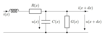
<p>A segment of a traditional transmission line is shown in the figure below. It
consists of a series distributed resistance \(R(x)\), inductance \(L(x)\) as well as
segment capacitance \(C(x)\) and conductance \(G(x)\). A transmission line is
thought of as a continuous series of these segments.</p>

<p><img src="https://journal.lunar.sh/images/7/transmission_line.png" alt="" /></p>

<p>It can be shown that the equations that describe changes in the voltage and
current on the line is given by:</p>

\[\frac{\partial u}{\partial x} dx = -Ri - L \frac{\partial i}{\partial t}\]

\[\frac{\partial i}{\partial x} dx = -Gu - C \frac{\partial u}{\partial t}\]

<p>The equations above are known as the telegrapher’s equations. These two
equations can be combined to produce two partial differential equations with one
isolated variable each (\({u}\) or \({i}\)).</p>

<p>\(u\) and \(i\) are related by the characteristic impedance (\(Z_{0}\)) of the
transmission line which can be derived from the telegraphers equations:</p>

\[Z_{0} = \frac{V^+(x)}{I^+(x)} = \sqrt{\frac{R(x)+j\omega L(x)}{G(x)+j\omega
C(x)}}\]

<p>For most transmission lines dielectric and conductor losses are low, so we
assume:</p>

\[R(x) \ll j\omega L(x), G(x) \ll j\omega C(x)\]

<p>As a result the equation above simplifies to:</p>

\[Z_{0} = \sqrt{\frac{L(x)}{C(x)}}\]

<p>It is worth noting that characteristic impedance \(Z_{0}\) of a transmission line
only has an effect at <code class="language-plaintext highlighter-rouge">RF</code> frequencies. It is not possible to measure the
characteristic impedance of a transmission line directly with a multimeter
because resistance (ohms law) and characteristic impedance (electromagnetic
property) are not the same concept.</p>

<p>Examples of transmission lines include coaxial cable and microstrip line.
Transmission lines typically have a characteristic impedance of <code class="language-plaintext highlighter-rouge">50</code> \(\Omega\) in
<code class="language-plaintext highlighter-rouge">RF</code> systems and are used to carry <code class="language-plaintext highlighter-rouge">RF</code> signals from one point in a circuit to
another with minimal losses.</p>

<h1 id="impedance-matching">Impedance Matching</h1>

<p>It is often said that impedance matching is what truly differentiates <code class="language-plaintext highlighter-rouge">RF</code> circuit
design from low frequency circuit design. Indeed, it is one of the most common
tasks for an <code class="language-plaintext highlighter-rouge">RF</code> designer.</p>

<p><code class="language-plaintext highlighter-rouge">RF</code> signals travelling along a transmission line can be thought of as
electromagnetic power waves. Power waves are a hypothetical construct, one of
the many possible linear transformations of voltage and current.</p>

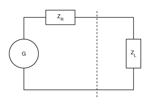
<p>The figure below shows a typical <code class="language-plaintext highlighter-rouge">RF circuit</code> consisting of a <code class="language-plaintext highlighter-rouge">RF</code> power source
(\(G\)) with an impedance of (\(Z_{R}\)) and a load with an impedance of \(Z_{L}\).
The interface of the generator and load impedance is indicated by the dotted
line.</p>

<p><img src="https://journal.lunar.sh/images/7/impedance_match.png" alt="" /></p>

<p>It is at this interface that we experience reflection of the power wave (back to
the generator) when \(Z_{R} \neq Z_{L}\). If the impedance of the generator and
load were equal then no reflection occurs.</p>

<p>In general, the goal of an <code class="language-plaintext highlighter-rouge">RF</code> system is to transfer <code class="language-plaintext highlighter-rouge">RF</code> power as efficiently from
one point to another with minimal reflections. The degree of an electromagnetic
power wave reflected (at the boundary) is determined by the reflection
coefficient (\(\Gamma\)):</p>

\[\Gamma_{L} = \frac{Z_{L} - Z_{0}}{Z_{L}+Z_{0}}\]

<p>A \(\Gamma\) of \(0\) indicates no reflection, while a \(\Gamma\) of <code class="language-plaintext highlighter-rouge">1</code> or <code class="language-plaintext highlighter-rouge">-1</code>
represents total reflection with or without phase inversion.</p>

<p>Here (\(Z_{0}\)) represents the reference impedance of the system which is
typically <code class="language-plaintext highlighter-rouge">50</code> \(\Omega\). Maximum power transfer over the boundary from the
generator to the load is only satisfied when:</p>

\[Z_{L} = Z_{R}^*\]

<p>This expression is known as the conjugate match rule for maximum power transfer.
In most practical <code class="language-plaintext highlighter-rouge">RF</code> systems \(Z_{L} \neq Z_{R}\) and so a method of impedance
transformation is required to satisfy the conjugate match rule.</p>

<p>Impedance transformation networks allow a \(Z_{L}\) with both a real and imaginary
part to be transformed into another complex impedance using reactive components.
Reactive components do not dissipate real power unlike resistors which is why
resistors are rarely used in <code class="language-plaintext highlighter-rouge">RF</code> impedance matching and filter networks.</p>

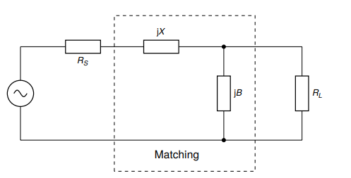
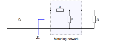
<p>The most basic type of impedance transformation network is known as the <code class="language-plaintext highlighter-rouge">LC</code>
network which consists of an inductor and capacitor. It can be used to transform
a complex load (\(R_{L}\)) to <code class="language-plaintext highlighter-rouge">50</code> \(\Omega\). The figure below shows the basic
configuration of the <code class="language-plaintext highlighter-rouge">LC</code> impedance transformation network.</p>

<p><img src="https://journal.lunar.sh/images/7/LC_match.png" alt="" /></p>

<p>In addition to the <code class="language-plaintext highlighter-rouge">LC</code> network’s impedance transformation property, the <code class="language-plaintext highlighter-rouge">LC</code>
network can have a low-pass or high-pass response depending on the shunt element
(\(jB\)). If it is capacitive then the <code class="language-plaintext highlighter-rouge">LC</code> network will have a low-pass response or
a high-pass response if it is inductive.</p>

<p>Typically the low pass configuration (with a shunt capacitor) is desired.</p>

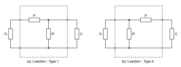
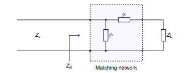
<p>It should be noted that the shunt element (\(jB\)) should be placed on the side
with the largest impedance. Therefore there are two possible configurations of
this network:</p>

<p><img src="https://journal.lunar.sh/images/7/LC_match_types.png" alt="" /></p>

<p>So that type <code class="language-plaintext highlighter-rouge">1</code> is used when \(R_{L} &gt; R_{S}\) and type <code class="language-plaintext highlighter-rouge">2</code> is used when \(R_{L} &lt;
R_{S}\). Here \(Z_{S}\) represents \(Z_{0}\) the system reference impedance \((50
\Omega)\).</p>

<p>The design procedure for a type <code class="language-plaintext highlighter-rouge">1</code> <code class="language-plaintext highlighter-rouge">LC</code> network is as follows. First we evaluate
the input impedance (\(Z_{in}\)) looking into the matching network.</p>

<p><img src="https://journal.lunar.sh/images/7/LC_match_type_1.png" alt="" /></p>

<p>We start by defining a few variables. Let:</p>

\[Z_{L} = R_{L} + jX_{L}\]

\[Z_{S} = Z_{0} = 50 \Omega\]

\[Z_{in} = jX + \frac{1}{(jB)^{-1} + (Z_{L})^{-1}}\]

<p>Matching conditions are met when \(Z_{in} = Z_{S} = Z_{0}\).</p>

<p>The equation above can be simplified and separated into real and imaginary
parts:</p>

\[B(X + X_{L}) = -(Z_{0}R_{L}-XX_{L})\]

\[B(R_{L} - Z_{0}) = Z_{0}X_{L} - R_{L}X\]

<p><code class="language-plaintext highlighter-rouge">B</code> can then be solved using the following equation:</p>

\[B = -\frac{R_{L}^2+X_{L}^2}{X_{L} + \sqrt{\frac{R_{L}}{Z_{0}}} \sqrt{R_{L}^2 + X_{L}^2 - Z_{0}R_{L}}}\]

<p>Once <code class="language-plaintext highlighter-rouge">B</code> is obtained, X may be found by rearranging for <code class="language-plaintext highlighter-rouge">X</code>:</p>

\[X = \frac{B(R_{L} - Z_{0}) - Z_{0}X_{L}}{-R_{L}}\]

<p>The figure below depicts the second variant of the <code class="language-plaintext highlighter-rouge">LC</code> matching network.</p>

<p><img src="https://journal.lunar.sh/images/7/LC_match_type_2.png" alt="" /></p>

<p>Let:</p>

\[Z_{L} = R_{L} + jX_{L}\]

\[Z_{S} = Z_{0} = 50 \Omega\]

\[Z_{in} = \frac{1}{(jB)^{-1} + (Z_{L} + jX)^{-1}}\]

<p>Matching conditions are met when \(Z_{in} = Z_{S} = Z_{0}\).</p>

<p>The equation above can be simplified and separated into real and imaginary
parts:</p>

\[B(X_{L} + X) = -Z_{0}R_{L}\]

\[B(Z_{0} - R_{L}) = -Z_{0}(X_{L}+X)\]

<p>Again, B can then be solved using the following equation:</p>

\[B = -Z_{0}\sqrt{\frac{R_{L}}{Z_{0}- R_{L}}}\]

<p>Again, <code class="language-plaintext highlighter-rouge">X</code> may be found by rearranging for \((X_{L} + X)\) and substituting to
yield:</p>

\[X = \sqrt{R_{L}(Z_{0} - R_{L})} - X_{L}\]

<p>For both <code class="language-plaintext highlighter-rouge">LC</code> circuit types it is assumed that \(jB\) represents a capacitive
element and \(jX\) represents an inductive element so that a low-pass response is
obtained.</p>

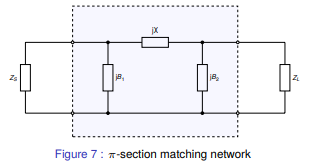
<p>Matching networks with more than two reactive elements also exist. These include
the \(\pi\)-section and <code class="language-plaintext highlighter-rouge">T-section</code> matching networks that contain <code class="language-plaintext highlighter-rouge">3</code> reactive
elements each. The figure below depicts the \(\pi\)-section network.</p>

<p><img src="https://journal.lunar.sh/images/7/pi_match.png" alt="" /></p>

<p>The \(\pi\)-section network is made up of a type <code class="language-plaintext highlighter-rouge">2</code> <code class="language-plaintext highlighter-rouge">LC</code> matching network in cascade
with a type 1 <code class="language-plaintext highlighter-rouge">LC</code> matching network. The central element \(jX\) is the sum of the
inductive reactance (\(jX\)) of each <code class="language-plaintext highlighter-rouge">LC</code> matching section, which is combined into a
single reactance.</p>

<p>A virtual load resistance \(R_{x}\) is interposed in-between the two <code class="language-plaintext highlighter-rouge">LC</code> matching
networks. The goal of the first <code class="language-plaintext highlighter-rouge">LC</code> matching network is to then match the source
\(Z_{S}\) to \(R_{x}\) while the second <code class="language-plaintext highlighter-rouge">LC</code> matching network matches \(R_{x}\) to
\(Z_{L}\).</p>

<p>The value of \(R_{x}\) is chosen according to the desired <code class="language-plaintext highlighter-rouge">Q-factor</code> and must be
smaller than \(R_{L}\) and \(R_{S}\). The <code class="language-plaintext highlighter-rouge">Q-factor</code> of a matching network describes
how well power is transferred from source to load as you deviate from the
designed center frequency of the matching network (\(f_{0}\)).</p>

<p>Is it defined as follows:</p>

\[Q = \frac{f_{0}}{B}\]

<p>Here \(f_{0}\) represents the center frequency of the matching network and B
represents the total bandwidth over which no greater than <code class="language-plaintext highlighter-rouge">3dB</code> of power is lost
from source to load.</p>

<p>A high <code class="language-plaintext highlighter-rouge">Q-factor</code> is often desirable for a narrowband matching network. It should
be mentioned that the <code class="language-plaintext highlighter-rouge">Q-factor</code> cannot be controlled with a simple 2 element <code class="language-plaintext highlighter-rouge">LC</code>
matching network (which id determined by \(R_{L}\) and \(R_{S}\)). This is one of
the advantages of the \(\pi\)-section matching network.</p>

<p>The <code class="language-plaintext highlighter-rouge">Q-factor</code> for the \(\pi\)-section filter is given by:</p>

\[Q_{\pi} = \sqrt{\frac{\max(R_{S}, R_{L})}{R_{x}} - 1}\]

<p>Here <code class="language-plaintext highlighter-rouge">max()</code> is a function that returns the maximum of two values. Hence the
<code class="language-plaintext highlighter-rouge">Q-factor</code> of a \(\pi\)-section matching network will be determined by the <code class="language-plaintext highlighter-rouge">LC</code>
matching section with the highest <code class="language-plaintext highlighter-rouge">Q-factor</code>.</p>

<h1 id="electromagnetic-transducers">Electromagnetic Transducers</h1>

<p>Once the necessary <code class="language-plaintext highlighter-rouge">RF</code> power has been generated and transmitted over various
transmission lines and matching networks it then becomes necessary to convert
this <code class="language-plaintext highlighter-rouge">RF</code> power into electromagnetic waves which can start propagating through
free space to reach a receiver. For this purpose we use an electromagnetic
transducer known as an antenna.</p>

<p>An antenna can be also be thought of as an impedance transformation network that
matches an <code class="language-plaintext highlighter-rouge">RF</code> circuit (<code class="language-plaintext highlighter-rouge">50</code> \(\Omega\) typical) to free space (<code class="language-plaintext highlighter-rouge">377</code> \(\Omega\)).</p>

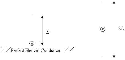
<p>An antenna can be as simple as a piece of wire connected to an <code class="language-plaintext highlighter-rouge">RF</code> output port
but the efficiency of the antenna in this case would be very low. The two most
common types of antenna’s are the <code class="language-plaintext highlighter-rouge">monopole</code> and <code class="language-plaintext highlighter-rouge">dipole</code> antenna (shown below).</p>

<p><img src="https://journal.lunar.sh/images/7/monopole_dipole.png" alt="" /></p>

<p>The <code class="language-plaintext highlighter-rouge">monopole</code> antenna consists of a <code class="language-plaintext highlighter-rouge">quarter-wave</code> length (\(\lambda/4\)) of wire of
length \(L\) which is connected to the ‘hot’ <code class="language-plaintext highlighter-rouge">RF</code> input terminal and a infinitely
large <code class="language-plaintext highlighter-rouge">RF</code> ground plane conductor which is connected to electrical ground. The
‘hot’ and <code class="language-plaintext highlighter-rouge">RF</code> ground elements are electrically separated from each other.</p>

<p>Most practical <code class="language-plaintext highlighter-rouge">HF</code> and <code class="language-plaintext highlighter-rouge">VHF</code> <code class="language-plaintext highlighter-rouge">monopole</code> antennas are shorter than a quarter
wavelength due to size constraints and are therefore modelled as electrically
small <code class="language-plaintext highlighter-rouge">monopoles</code> (\(L \leq (1/8)\lambda\)) from this point forward.</p>

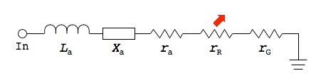
<p>An electrically small <code class="language-plaintext highlighter-rouge">monopole</code> antenna can be modelled as a series circuit with
the elements shown in the image below.</p>

<p><img src="https://journal.lunar.sh/images/7/antenna_model.jpg" alt="" /></p>

<p>\(L_{a}\) represents the antenna conductor inductance. This is the parasitic
inductance of the active element of the antenna which is just a wire made out of
a material such as copper with a length and diameter. This value is usually very
small and can be neglected.</p>

<p>The reactance of an electrically short <code class="language-plaintext highlighter-rouge">monopole</code> (\(L \leq (1/8)\lambda\)) is
represented by \(X_{a}\) and can be calculated as follows:</p>

\[X_{a} = 60(1 - \ln{(\frac{L}{a})})\cot{(2\pi\frac{L}{\lambda})}j \Omega\]

<p>This equation originally appears in the “Antenna Engineering Handbook”, Third
Edition by <code class="language-plaintext highlighter-rouge">Richard C. Johnson</code>.</p>

<p>From the equation above it can be seen that the reactance of an electrically
short <code class="language-plaintext highlighter-rouge">monopole</code> is primarily capacitive.</p>

<p>The radius of the wire (active element) in meters is given by \(a\) and the
operational wavelength is given by \(\lambda\). The operational wavelength can be
calculated by the transmit frequency (\(f_{t}\)) and the speed of light in a
vacuum (\(c\)):</p>

\[\lambda = \frac{c}{f_{t}}\]

<p>The loss resistance \(r_{a}\) is the effective ac resistance of the antenna active
element due to the skin effect. The skin effect is a phenomenon whereby <code class="language-plaintext highlighter-rouge">RF</code>
current tends to flow near the surface of the conductor as the frequency, and as
a consequence, magnetic field strength at the center of the conductor increases.</p>

<p>The skin depth is given by:</p>

\[\delta = \frac{1}{\sqrt{\pi f_{t} \mu_{0} \sigma}}\]

<p>\(\sigma\) is the conductivity of the active element’s composite material (copper)
while \(\mu_{0}\) is the permeability constant. Once \(\sigma\) is computed the real
ac resistance can be found as follows:</p>

\[r_{a} = \frac{L}{2\pi a \delta \sigma}\]

<p>At <code class="language-plaintext highlighter-rouge">VHF</code> the loss resistance \(r_{a}\) is also very small and can typically be
neglected.</p>

<p>The radiation resistance \(r_{R}\) of an electrically small monopole (\(L \leq
(1/8)\lambda\)) is the effective real resistance that represents the power that
is radiated away from the antenna as electromagnetic waves. For an electrically
short <code class="language-plaintext highlighter-rouge">monopole</code>, radiation resistance is given by the equation below:</p>

\[r_{R} = 40 \pi^2(\frac{L}{\lambda})^2 \Omega\]

<p>\(r_{G}\) represents the losses in the <code class="language-plaintext highlighter-rouge">RF</code> ground plane and this parameter is
usually neglected. A stable <code class="language-plaintext highlighter-rouge">RF</code> ground plane is essential for an antenna to
function correctly. An antenna ground plane serves as an <code class="language-plaintext highlighter-rouge">RF</code> return path for <code class="language-plaintext highlighter-rouge">AC</code>
displacement current.</p>

<p>For a <code class="language-plaintext highlighter-rouge">monopole</code> the ground plane also serves the function of mirroring the active
radiation element to form the second half of the antenna. This derivation is
obtained using image theory and is beyond the scope of this journal entry.</p>

<h1 id="s-parameters">S-Parameters</h1>

<p>Most passive <code class="language-plaintext highlighter-rouge">RF</code> circuits such as filters, matching networks, etc are linear.
That is their output voltage, current and power relationships are derived from a
system of linear equations. Some active devices such as <code class="language-plaintext highlighter-rouge">class-A</code> <code class="language-plaintext highlighter-rouge">small-signal</code>
amplifiers are also linear.</p>

<p>Scattering parameters or <code class="language-plaintext highlighter-rouge">S-parameters</code> can be used to model the behaviour of
these <code class="language-plaintext highlighter-rouge">linear</code> <code class="language-plaintext highlighter-rouge">RF</code> networks when stimulated by a steady-state signal.</p>

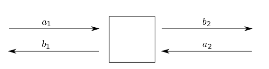
<p><img src="https://journal.lunar.sh/images/7/s_param.png" alt="" /></p>

<p>The image above depicts a <code class="language-plaintext highlighter-rouge">DUT</code> ‘black box’ which we use to derive the scattering
parameters. The network has <code class="language-plaintext highlighter-rouge">2</code> distinct ports (<code class="language-plaintext highlighter-rouge">port 1</code>, <code class="language-plaintext highlighter-rouge">port 2</code>) and 4 scattering
parameters: \(S_{11}, S_{12}\) and \(S_{21}, S_{22}\). The scattering parameters are
complex values with both a real and imaginary part.</p>

<p>We define each scattering parameter in terms of two voltage waves at the input
(<code class="language-plaintext highlighter-rouge">port 1</code>) and output (<code class="language-plaintext highlighter-rouge">port 2</code>). Let \(a_{1}, b_{1}\) represents the incident and
reflected voltage waves at <code class="language-plaintext highlighter-rouge">port 1</code> while \(a_{2}, b_{2}\) represent the incident
and reflected voltage waves at <code class="language-plaintext highlighter-rouge">port 2</code>.</p>

<p>The S-parameters can then be defined as follows:</p>

\[S_{11} = \frac{b_{1}}{a_{1}} = \frac{V_{1}^-}{V_{1}^+}, S_{12} =
\frac{b_{1}}{a_{2}} = \frac{V_{1}^-}{V_{2}^+}\]

\[S_{21} = \frac{b_{2}}{a_{1}} = \frac{V_{2}^-}{V_{1}^+}, S_{22} =
\frac{b_{2}}{a_{2}} = \frac{V_{2}^-}{V_{2}^+}\]

<p>It should be mentioned at this point that s-parameters can also be defined in
terms of ‘power waves’ by considering the complex input impedance of the <code class="language-plaintext highlighter-rouge">DUT</code>.
However the voltage wave definition is the most popular.</p>

<p>A system of linear equations can then be derived for \(b_{1}\) and \(b_{2}\):</p>

\[b_{1} = S_{11}a_{1} + S_{12}a_{2}\]

\[b_{2} = S_{21}a_{1} + S_{22}a_{2}\]

<p>Which can be expressed in terms of the <code class="language-plaintext highlighter-rouge">S-parameter</code> matrix:</p>

\[\begin{bmatrix} b_{1} \\
b_{2} \end{bmatrix} \begin{bmatrix} S_{11} S_{12} \\
S_{21}  S_{22} \end{bmatrix} = \begin{pmatrix}  a_{1} \\
a_{2} \end{pmatrix}\]

<p>There are various useful definitions that can be derived from the scattering
parameters. \(S_{21}\) and \(S_{11}\) are the most commonly used scattering
paramters.</p>

<p>The first useful definition is the logarithmic power gain of the network in <code class="language-plaintext highlighter-rouge">dB</code>
(\(G_{p}\)) which can be expressed in terms of \(|S_{21}|\):</p>

\[G_{p} = 20\log_{10}|S_{21}|\]

<p>\(S_{11}\) is related to the input reflection coefficient \(\Gamma_{in}\) and can be
used to obtain the input impedance of the network \(Z_{in}\):</p>

\[S_{11} = \Gamma_{in}\]

\[Z_{in} = Z_{0} \frac{1+S_{11}}{1-S_{11}}\]

<p>The ratio of reflected (\(P_{ref}\)) and incident power (\(P_{inc}\)) at <code class="language-plaintext highlighter-rouge">port 1</code> is
given by:</p>

\[\frac{P_{ref}}{P_{inc}} = |\Gamma_{in}|^2\]

<p>Another useful definition is the input (<code class="language-plaintext highlighter-rouge">port 1</code>) return loss \(RL_{in}\):</p>

\[RL_{in} = -20\log_{10}(|S_{11}|)\]

<p>From the above formula it can be seen that return loss is typically a positive
number (since \(|S11| &lt; 0\)), however sometimes it is quoted as a negative number
in which case the data is referring to the <code class="language-plaintext highlighter-rouge">log</code> magnitude of \(S_{11}\) directly
(\(-RL_{in}\)), not the actual return loss which is positive as mentioned.</p>

<p>Return loss for (\(S_{11}\)) is a measure of how well matched <code class="language-plaintext highlighter-rouge">port 1</code> of the
network is to the reference impedance. A return loss greater than <code class="language-plaintext highlighter-rouge">10dB</code> is
usually desirable for a good match.</p>

<p>Another measure of how well matched a network is to the reference impedance is
called <code class="language-plaintext highlighter-rouge">VSWR</code> (voltage standing wave ratio). The <code class="language-plaintext highlighter-rouge">VSWR</code> of <code class="language-plaintext highlighter-rouge">port 1</code> (\(s_{in}\)) is
defined by:</p>

\[s_{in} = \frac{1+|S_{11}|}{1-|S_{11}|}\]

<p><code class="language-plaintext highlighter-rouge">VSWR</code> is typically used to measure the matching conditions of antennas. A
(\(s_{in} &lt; 2\)) is generally considered suitable for most antenna applications.</p>

<p>A <code class="language-plaintext highlighter-rouge">VNA</code> (Vector Network Analyzer) is an instrument that is used to measure
<code class="language-plaintext highlighter-rouge">S-parameters</code>. Most affordable commercial <code class="language-plaintext highlighter-rouge">VNA's</code> are <code class="language-plaintext highlighter-rouge">2-port</code> <code class="language-plaintext highlighter-rouge">1-path</code> devices, i.e
they only measure \(S_{11}\) and \(S_{21}\) and the <code class="language-plaintext highlighter-rouge">DUT</code> must therefore be reversed
to obtain \(S_{22}\) and \(S_{12}\).</p>

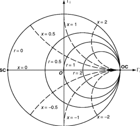
<p>The input and output impedance obtained for \(S_{11}\) and \(S_{22}\) can also be
represented in graphical form as a smith chart. A <code class="language-plaintext highlighter-rouge">smith chart</code> is a real and
imaginary chart where the imaginary (<code class="language-plaintext highlighter-rouge">y-axis</code>) axis has been bent around the
<code class="language-plaintext highlighter-rouge">x-axis</code>. It can be used to plot any value of complex impedance. An example of the
<code class="language-plaintext highlighter-rouge">smith chart</code> is shown in the figure below.</p>

<p>The top half of the smith chart represent inductive reactance while the bottom
half represents capacitive reactance. The circles passing through the <code class="language-plaintext highlighter-rouge">x-axis</code> are
known as constant resistance circles where the left most point on the real axis
of the smith chart represents a short circuit (<code class="language-plaintext highlighter-rouge">SC</code>) while the rightmost point
represents an open circuit (<code class="language-plaintext highlighter-rouge">OC</code>).</p>

<p>For an ideal <code class="language-plaintext highlighter-rouge">50</code> \(\Omega\) match there should be a single point in the middle of
the smith chart.</p>

<p><img src="https://journal.lunar.sh/images/7/smith_chart.png" alt="" height="300px" /></p>

<h1 id="harmonic-balance">Harmonic Balance</h1>

<p><code class="language-plaintext highlighter-rouge">RF</code> power amplifier’s are <code class="language-plaintext highlighter-rouge">large-signal</code> non-linear devices.</p>

<p>At this point a distinction is required between small signal and large signal
amplifiers. For <code class="language-plaintext highlighter-rouge">small-signal</code> amplifiers the input and output power is typically
small and these devices typically operate in their <code class="language-plaintext highlighter-rouge">linear</code> region.</p>

<p><code class="language-plaintext highlighter-rouge">Large-signal</code>, <code class="language-plaintext highlighter-rouge">class AB</code>, <code class="language-plaintext highlighter-rouge">B</code> and <code class="language-plaintext highlighter-rouge">C</code> devices typically operate with large input and
output power and their response is strongly <code class="language-plaintext highlighter-rouge">non-linear</code> due to the class of
operation. Therefore for power amplifier classes other than <code class="language-plaintext highlighter-rouge">class A</code>,
<code class="language-plaintext highlighter-rouge">S-parameters</code> cannot be used reliably in the design of <code class="language-plaintext highlighter-rouge">RF</code> power amplifiers.</p>

<p>Rather a designer relies on vendor supplied <code class="language-plaintext highlighter-rouge">non-linear</code> software models of the
power amplifier transistor and typically uses a <code class="language-plaintext highlighter-rouge">non-linear</code> frequency domain
analysis technique such as the harmonic balance method (<code class="language-plaintext highlighter-rouge">HBM</code>) to characterise the
power amplifier’s performance.</p>

<p><code class="language-plaintext highlighter-rouge">Harmonic balance</code> is a frequency domain technique used to calculate the steady
state response of a non-linear circuit. <code class="language-plaintext highlighter-rouge">HBM</code> can be defined in multiple ways,
however in this case let us demonstrate <code class="language-plaintext highlighter-rouge">HBM</code> through an example circuit.</p>

<p>Given a circuit with \(N\) nodes, let vector \(v\) represent the respective node
voltages. For ease of representation we model a circuit with capacitors and
voltage controlled resistors. Then applying <code class="language-plaintext highlighter-rouge">KCL</code> (Kirchoff’s Current Law) to the
circuit yields the following systems of equations:</p>

\[f(v,t) = i(v(t)) + \frac{d}{dt}q(v(t)) + \int_{-\infty}^t{y(t-\tau)v(\tau)} +
i_{s}(t) = 0\]

<p>We let \(q\) and \(i\) represent the sum of the charges and currents entering the
nodes due to the non-linearities. \(y\) is the impulse response matrix of the
circuit with all non-linearities removed while \(i_{s}\) represents the external
source currents.</p>

<p>We then convert equation above into the frequency domain:</p>

\[F(V) = I(V) + ZQ(V) + YV + I_{s} = 0\]

<p>Here \(Z\) represents a matrix with frequency coefficients representing the
differentiation step. The convolution integral in the equation above maps to <code class="language-plaintext highlighter-rouge">YV</code>
as shown where <code class="language-plaintext highlighter-rouge">Y</code> is the admittance matrix for the <code class="language-plaintext highlighter-rouge">linear</code> portion of the circuit.</p>

<p><code class="language-plaintext highlighter-rouge">V</code> then contains the fourier coefficients of the voltage at each \(N\) nodes at
every harmonic. This process is merely nothing more than <code class="language-plaintext highlighter-rouge">KCL</code> in the frequency
domain for <code class="language-plaintext highlighter-rouge">non-linear</code> circuits.</p>

<h1 id="lumped-and-distributed-element-networks">Lumped and Distributed Element Networks</h1>

<p>As mentioned above, as the size of a circuit element starts to approach a
fraction (typically <code class="language-plaintext highlighter-rouge">1/10</code>) of the wavelength of the highest <code class="language-plaintext highlighter-rouge">RF</code> signal frequency,
the lumped element approximation for the circuit element no longer holds. In
these cases lumped or discrete components cannot be used and so a distributed
element/model must be utilized.</p>

<p>Traditionally the use of lumped element components at <code class="language-plaintext highlighter-rouge">RF</code> frequencies is most
common below around <code class="language-plaintext highlighter-rouge">500 MHz</code>. Above <code class="language-plaintext highlighter-rouge">500 MHz</code> these lumped circuit
elements become more difficult to design with.</p>

<h1 id="classes-of-operation">Classes Of Operation</h1>

<p>Depending on the <code class="language-plaintext highlighter-rouge">DC</code> operating point of the power transistor, different values of
efficiency and output power can be obtained for the same input power. Efficiency
is generally considered the most important design parameter for an <code class="language-plaintext highlighter-rouge">RF</code> power
amplifier.</p>

<p>In the <code class="language-plaintext highlighter-rouge">class-A</code> configuration the transistor is biased such that the quiescent
drain current is equal to the peak amplitude of the current expected through the
load. This allows for a symmetrical voltage and current swing at the output and
the transistor conducts for the full <code class="language-plaintext highlighter-rouge">360</code> degrees of the input waveform.</p>

<p>The advantages of this configuration are excellent linearity and gain at the
expense of reduced efficiency. A <code class="language-plaintext highlighter-rouge">class-A</code> power amplifier with an inductively
loaded drain has a maximum theoretical efficiency of <code class="language-plaintext highlighter-rouge">50%</code>.</p>

<p><code class="language-plaintext highlighter-rouge">Class-B</code> power amplifiers aim to achieve greater efficiency by only conducting
for half of the input drive cycle (<code class="language-plaintext highlighter-rouge">180</code> degrees). <code class="language-plaintext highlighter-rouge">Class-B</code> power amplifiers have a
maximum theoretical efficiency of <code class="language-plaintext highlighter-rouge">75%</code> and the transsitor is biased at cutoff.
Again <code class="language-plaintext highlighter-rouge">class-B</code> <code class="language-plaintext highlighter-rouge">PA's</code> can be placed in a single-ended configuration or push-pull.
The advantage of <code class="language-plaintext highlighter-rouge">class-B</code> are increased efficiency at the expense of decreased
linearity.</p>

<p>A compromise is thus needed between <code class="language-plaintext highlighter-rouge">class A</code> and <code class="language-plaintext highlighter-rouge">class B</code> such that we have
sufficient linearity at a reasonable efficiency. A <code class="language-plaintext highlighter-rouge">class-AB</code> power amplifier is a
solution to this problem.</p>

<p>In the <code class="language-plaintext highlighter-rouge">class-AB</code> mode of operation the transistor is biased with a quiescent
drain current slightly to moderately above cutoff, depending on the linearity
requirements. This improves the linearity of the power amplifier while typically
maintaining an efficiency of <code class="language-plaintext highlighter-rouge">50%</code> to <code class="language-plaintext highlighter-rouge">70%</code> in practice. <code class="language-plaintext highlighter-rouge">Class-AB</code> power
amplifier’s have a conduction angle between <code class="language-plaintext highlighter-rouge">180</code> and <code class="language-plaintext highlighter-rouge">360</code> degrees.</p>

<p>The <code class="language-plaintext highlighter-rouge">single-ended</code>, <code class="language-plaintext highlighter-rouge">class-AB</code> mode of operation is therefore a popular choice
amongst designers.</p>

<h1 id="stability-analysis">Stability Analysis</h1>

<p><code class="language-plaintext highlighter-rouge">RF</code> power
amplifier’s are inherently unstable devices which often require some form of
stabilization to operate correctly.</p>

<p>Amplifier instability is usually caused by some type of gain and feedback
mechanism. In <code class="language-plaintext highlighter-rouge">MOSFET</code> transistor’s the feedback mechanism is typically due to the
gate to drain capacitance that couples a portion of the output back into the
input and vice versa. This effect often manifests as unwanted oscillation at
either the input and output of the PA.</p>

<p>Small signal parameters (such as <code class="language-plaintext highlighter-rouge">S-parameters</code>) are typically used to
characterize stability of <code class="language-plaintext highlighter-rouge">RF</code> power amplifier’s even though these are <code class="language-plaintext highlighter-rouge">non-linear</code>
devices. This is because small signal models can still provide useful insights
into the design of a <code class="language-plaintext highlighter-rouge">PA</code> without requiring complex non-linear calculations.
Typically the operation of a <code class="language-plaintext highlighter-rouge">PA</code> is linearized around an operating point.</p>

<p>There are various stability factors available to a designer and an amplifier may
be conditionally stable or unconditionally stable. If an amplifier is
conditionally stable then there exists a load and source impedance that causes
the amplifier to oscillate. Therefore unconditional stability is usually
desired.</p>

<p>The most common stability factor in use is the <code class="language-plaintext highlighter-rouge">Rollet</code> stability factor (\(K\))
which is defined as follows:</p>

\[K = \frac{1 - |S_{11}|^2 - |S_{22}|^2 + | \Delta |^2}{2|S_{12}S_{21}|}\]

<p>Here \(\|\Delta\|\) is defined as the scattering-matrix determinant:</p>

\[| \Delta | = |S_{11}S_{22} - S_{21}S_{12}|\]

<p>We define three more stability Criterion in terms of \(\Delta, B_{1}\) and
\(B_{2}\):</p>

\[B_{1} = 1 + |S_{11}|^2 - |S_{22}|^2 - |\Delta|^2\]

\[B_{2} = 1 + |S_{22}|^2 - |S_{11}|^2 - |\Delta|^2\]

<p>In order for an amplifier to be conditionally stable we require the
following conditions:</p>

\[K \ge 1\]

\[\Delta &lt; 1\]

\[B_{1} &gt; 0, B_{2} &gt; 0\]

<h1 id="efficiency">Efficiency</h1>
<p>The most common measure of <code class="language-plaintext highlighter-rouge">RF</code> power amplifier efficiency is \(PAE\)
(power added efficiency) and is defined as follows:</p>

\[PAE = \frac{P_{out} - P_{in}}{P_{DC}}\]

<p>Here \(P_{in}\) represents the <code class="language-plaintext highlighter-rouge">RF</code> input power from the source, \(P_{out}\)
represents <code class="language-plaintext highlighter-rouge">RF</code> power delivered to the load and \(P_{DC}\) represents the total <code class="language-plaintext highlighter-rouge">DC</code>
power.</p>

<h1 id="p1db-compression-point">P1dB Compression Point</h1>

<p>The <code class="language-plaintext highlighter-rouge">P1dB</code> point is defined as the output power level at which
the gain of an amplifier decreases by <code class="language-plaintext highlighter-rouge">1 dB</code> from its nominal value which
indicates the onset of gain non-linearity.</p>

<p>Most amplifier’s start to compress  approximately <code class="language-plaintext highlighter-rouge">5</code> to <code class="language-plaintext highlighter-rouge">10 dB</code> below their <code class="language-plaintext highlighter-rouge">P1dB</code>
point.</p>

<p>The <code class="language-plaintext highlighter-rouge">P1dB</code> point indicates that power amplifier’s have a linear and non-linear
region of power gain.</p>

<h1 id="load-pull">Load Pull</h1>

<p><code class="language-plaintext highlighter-rouge">Load-pull</code> is an empirical <code class="language-plaintext highlighter-rouge">RF</code> <code class="language-plaintext highlighter-rouge">PA</code> design technique in which the
reflection coefficient or impedance presented to the drain of a <code class="language-plaintext highlighter-rouge">RF</code> power
transistor is varied by an electrical or mechanical impedance tuner to any
arbitrary value. The technique is traditionally used to determine the optimum
load impedance to present to an <code class="language-plaintext highlighter-rouge">RF</code> power amplifier for maximum output power.</p>

<p>Once the optimum load impedance is determined the synthesis of matching networks
can then take place. <code class="language-plaintext highlighter-rouge">Load-pull</code> tuners are expensive devices and are therefore
typically out of the reach of most students or experimenters.</p>

<p>In the case where a physical <code class="language-plaintext highlighter-rouge">load-pull</code> tuner is not available and a <code class="language-plaintext highlighter-rouge">non-linear</code>
model for the chosen <code class="language-plaintext highlighter-rouge">RF</code> power transistor exists, then a simulated <code class="language-plaintext highlighter-rouge">load-pull</code> can
be performed.</p>

<h1 id="lc-filtering">LC Filtering</h1>

<p>As <code class="language-plaintext highlighter-rouge">non-linear</code> devices, power amplifiers typically produce
harmonic frequency content that must be filtered out in order to comply with
regulatory standards on spurious emissions. <code class="language-plaintext highlighter-rouge">LC</code> networks can be constructed with
varying number of elements (poles) in order to achieve a specific roll-off in
the stop-band.</p>

<p>Two types of filter response are commonly used in <code class="language-plaintext highlighter-rouge">RF</code> circuit design, these are
the <code class="language-plaintext highlighter-rouge">Chebyshev</code> and <code class="language-plaintext highlighter-rouge">Butterworth</code> responses. <code class="language-plaintext highlighter-rouge">Chebyshev</code> <code class="language-plaintext highlighter-rouge">LC</code> filters typically have a
steeper roll-off but suffer from passband ripple.</p>

<p><code class="language-plaintext highlighter-rouge">Butterworth</code> <code class="language-plaintext highlighter-rouge">LC</code> filters typically have a flat response in the passband with a
gradual roll-off in the stop band. These types of filters can be designed
manually using filter constants or using <code class="language-plaintext highlighter-rouge">RF</code> design software such as <code class="language-plaintext highlighter-rouge">Matlab</code> (<code class="language-plaintext highlighter-rouge">RF
Toolbox</code>) and typically an optimization algorithm. We typically optomize for
either stopband attenuation or input impedance.</p>

<p>That concludes this journal entry! I have just touched on some basic principles that
might help with understanding more advanced concepts.</p>

<h1 id="signature">Signature</h1>

<div class="language-plaintext highlighter-rouge"><div class="highlight"><pre class="highlight"><code><table class="rouge-table"><tbody><tr><td class="rouge-gutter gl"><pre class="lineno">1
2
3
4
5
6
7
8
9
10
11
12
13
14
15
16
17
18
19
</pre></td><td class="rouge-code"><pre>+---------------------------------------+
|     .-.       .-.       .-.           |
|    /   \     /   \     /   \     +    |
|         \   /     \   /     \   /     |
|          "_"       "_"       "_"      |
|                                       |
|  _   _   _ _  _   _   ___   ___ _  _  |
| | | | | | | \| | /_\ | _ \ / __| || | |
| | |_| |_| | .` |/ _ \|   /_\__ \ __ | |
| |____\___/|_|\_/_/ \_\_|_(_)___/_||_| |
|                                       |
|                                       |
| Lunar RF Labs                         |
| Email: root@lunar.sh                  |
|                                       |
| Research Laboratories                 |
| OpenAlias (BTC, XMR): lunar.sh        |
| Copyright (C) 2022-2024               |
+---------------------------------------+
</pre></td></tr></tbody></table></code></pre></div></div>]]></content><author><name>Dylan Müller</name></author><summary type="html"><![CDATA[A short primer on some of the basic concepts related to RF circuit and RF power amplifier design.]]></summary></entry><entry><title type="html">A simple GSC loader for COD Black Ops 1</title><link href="https://journal.lunar.sh/2023/gsctool.html" rel="alternate" type="text/html" title="A simple GSC loader for COD Black Ops 1" /><published>2023-09-17T00:00:00+00:00</published><updated>2023-09-17T00:00:00+00:00</updated><id>https://journal.lunar.sh/2023/gsctool</id><content type="html" xml:base="https://journal.lunar.sh/2023/gsctool.html"><![CDATA[<blockquote>
  <p>Learn how <code class="language-plaintext highlighter-rouge">GSC</code> scripts are loaded into <a href="https://en.wikipedia.org/wiki/Call_of_Duty:_Black_Ops">Black Ops 1</a> and how to write your own
simple <code class="language-plaintext highlighter-rouge">GSC</code> loader in <code class="language-plaintext highlighter-rouge">C</code> for the Microsoft Windows version of the game.</p>
</blockquote>

<ol>
  <li><a href="#fond-memories">Fond Memories</a></li>
  <li><a href="#game-script-code">Game Script Code</a></li>
  <li><a href="#gsc-script-call-chain">GSC Script Call Chain</a></li>
  <li><a href="#format-of-raw-gsc-scripts">Format of raw GSC scripts</a></li>
  <li><a href="#loading-and-executing-gsc-script-assets">Loading and executing GSC script assets</a></li>
  <li><a href="#black-ops-offsets">Black Ops Offsets</a></li>
  <li><a href="#source-code">Source Code</a></li>
  <li><a href="#demo">Demo</a></li>
</ol>

<h1 id="fond-memories">Fond Memories</h1>

<p><img src="https://journal.lunar.sh/images/6/01.jpg" alt="Black Ops 1 Zombies" />
Call of Duty: Black Ops 1</p>

<p><code class="language-plaintext highlighter-rouge">Call of Duty: Black Ops 1</code> for Microsoft Windows was released all the back back
in 2010! At the time I was still a teenager in high-school and a dedicated
gamer.</p>

<p>It seemed like another purchase on steam back then but I would have never
expected a game to produce so many fond memories playing kino der toten zombies
with friends from all over the world.</p>

<p>I mean who doesn’t remember all the iconic glitches, mystery boxes, etc of the
game? Some say the <code class="language-plaintext highlighter-rouge">Black Ops 1</code> <code class="language-plaintext highlighter-rouge">zombies</code> was the best in the <code class="language-plaintext highlighter-rouge">Black Ops</code> series.
There is something about the game aesthetics that creates a rush of nostalgia
:video_game:.</p>

<blockquote>
  <p>Ok enough rambling, let’s get technical…</p>
</blockquote>

<h1 id="game-script-code">Game Script Code</h1>

<p><code class="language-plaintext highlighter-rouge">GSC</code> is an internal scripting language that is used to script missions and game
modes for <code class="language-plaintext highlighter-rouge">Black Ops 1</code>. It has a syntax similar to <code class="language-plaintext highlighter-rouge">C++</code> but is a very limited
language. Here is an example:</p>

<div class="language-plaintext highlighter-rouge"><div class="highlight"><pre class="highlight"><code><table class="rouge-table"><tbody><tr><td class="rouge-gutter gl"><pre class="lineno">1
2
3
4
5
6
7
8
9
10
11
12
13
14
15
16
17
18
19
20
21
22
23
24
25
26
27
</pre></td><td class="rouge-code"><pre>#include common_scripts\utility;
#include maps\_utility;

init()
{
	level thread on_player_connect();

	// TODO: put weapon init's here
	maps\_flashgrenades::main();
	maps\_weaponobjects::init();
	maps\_explosive_bolt::init();
	maps\_flamethrower_plight::init();
	maps\_ballistic_knife::init();
}

on_player_connect()
{
	while( true )
	{
		level waittill("connecting", player);

		player.usedWeapons = false;
		player.hits = 0;

		player thread on_player_spawned();
	}
}
</pre></td></tr></tbody></table></code></pre></div></div>

<p><code class="language-plaintext highlighter-rouge">GSC</code> scripts are only loaded and executed when a map or game has started and in
<code class="language-plaintext highlighter-rouge">Black Ops 1</code> they are reloaded every time a map or game mode is restarted. Writing
custom <code class="language-plaintext highlighter-rouge">GSC</code> scripts is thus the basis for the vast majority of <code class="language-plaintext highlighter-rouge">Black Ops 1</code>
modding efforts.</p>

<p><code class="language-plaintext highlighter-rouge">GSC</code> scripts are first loaded into memory and then compiled with an internal <code class="language-plaintext highlighter-rouge">GSC</code>
compiler. There is a public <code class="language-plaintext highlighter-rouge">GSC</code> compiler and decompiler on <code class="language-plaintext highlighter-rouge">GitHub</code>:
<a href="https://github.com/xensik/gsc-tool">gsc-tool</a> but support for <code class="language-plaintext highlighter-rouge">Black Ops 1 (T5)</code>
seems to be missing.</p>

<p>Luckily it turns out we don’t actually need an external <code class="language-plaintext highlighter-rouge">GSC</code> compiler to compile
our own <code class="language-plaintext highlighter-rouge">GSC</code> scripts. We can (in theory) simply call the <code class="language-plaintext highlighter-rouge">compile()</code> function of
the internal <code class="language-plaintext highlighter-rouge">GSC</code> compiler and pass our mod script.</p>

<p>Whenever we talk about hooking a function or calling an in-game function we
usually assume that static analysis has been performed on the game binary to
find functions and offsets of interest. <code class="language-plaintext highlighter-rouge">IDA Pro</code> is my disassembler of choice
but <code class="language-plaintext highlighter-rouge">Ghidra</code> is probably also worth mentioning.</p>

<p>For debugging, <code class="language-plaintext highlighter-rouge">Cheat Engine</code> usually does the job quite well. However debugging
<code class="language-plaintext highlighter-rouge">Black Ops 1</code> is not as simple as attaching to the process and setting
breakpoints.</p>

<p>As far as I know this was possible in the official release version of the game,
but the game received multiple updates/patches which introduced various
primitive <code class="language-plaintext highlighter-rouge">anti-debugging</code> and anti cheat detections which must be bypassed.</p>

<p>Usually if I am starting reverse engineering on a game, my first quick option is
<a href="https://github.com/nihilus/ScyllaHide">scyllahide</a>. This seemed to work
for the latest <code class="language-plaintext highlighter-rouge">Black Ops 1</code> patch which allowed me to set breakpoints in game
which aided in the search for various <code class="language-plaintext highlighter-rouge">Black Ops 1</code> function addresses.</p>

<p>As we know research is an important part of any reverse engineering task,
without adequate research you could be wasting hours, days or even months of
your time by doing the same work that others have done before.</p>

<p>So I started research and found out that the source code for the <code class="language-plaintext highlighter-rouge">CoD 4</code> server
was leaked at some point and can be found in the following repo:
<a href="https://github.com/callofduty4x/CoD4x_Server">cod4x_server</a></p>

<p>This is very valuable information and was the basis for understanding how <code class="language-plaintext highlighter-rouge">GSC</code>
scripts are loaded and compiled in game.</p>

<h1 id="gsc-script-call-chain">GSC Script Call Chain</h1>

<p>The next task was figuring out the call chain (sequence of function calls) which
is required for loading custom <code class="language-plaintext highlighter-rouge">GSC</code> scripts. So I decided to search for the
keyword <code class="language-plaintext highlighter-rouge">script</code> and stumbled upon a function called <code class="language-plaintext highlighter-rouge">Scr_LoadScript</code>
<a href="https://github.com/callofduty4x/CoD4x_Server/blob/14f0d8a205d80c9b30e308b57f0cd9bd6d7cdb1c/src/scr_vm_main.c#L1018">here</a>
which seemed to be responsible for loading a <code class="language-plaintext highlighter-rouge">GSC</code> or <code class="language-plaintext highlighter-rouge">CSC</code> script (<code class="language-plaintext highlighter-rouge">CSC</code> scripts are
almost identical to <code class="language-plaintext highlighter-rouge">GSC</code> scripts but are executed by the client instead of a
server).</p>

<p>The only argument to <code class="language-plaintext highlighter-rouge">Scr_LoadScript</code> was a const character string however:</p>

<div class="language-plaintext highlighter-rouge"><div class="highlight"><pre class="highlight"><code><table class="rouge-table"><tbody><tr><td class="rouge-gutter gl"><pre class="lineno">1
</pre></td><td class="rouge-code"><pre>unsigned int Scr_LoadScript(const char* scriptname)
</pre></td></tr></tbody></table></code></pre></div></div>

<p>which I assumed was some type of resource/asset string. I therefore proceeded to
look for any functions that would load assets and stumbled upon <code class="language-plaintext highlighter-rouge">DB_AddXAsset</code>
<a href="https://github.com/callofduty4x/CoD4x_Server/blob/14f0d8a205d80c9b30e308b57f0cd9bd6d7cdb1c/src/bspc/db_miniload.cpp#L2919">here</a>.</p>

<p>The function signature for <code class="language-plaintext highlighter-rouge">DB_addXAasset</code> was as follows:</p>

<div class="language-plaintext highlighter-rouge"><div class="highlight"><pre class="highlight"><code><table class="rouge-table"><tbody><tr><td class="rouge-gutter gl"><pre class="lineno">1
</pre></td><td class="rouge-code"><pre>XAssetHeader __cdecl DB_AddXAsset(XAssetType type, XAssetHeader header)
</pre></td></tr></tbody></table></code></pre></div></div>

<p>I decided to search for the definition of <code class="language-plaintext highlighter-rouge">XAssetHeader</code>. <code class="language-plaintext highlighter-rouge">XAssetHeader</code> was
defined as a union of various
<a href="https://github.com/callofduty4x/CoD4x_Server/blob/14f0d8a205d80c9b30e308b57f0cd9bd6d7cdb1c/src/xassets.h#L81">structs</a>:</p>

<div class="language-plaintext highlighter-rouge"><div class="highlight"><pre class="highlight"><code><table class="rouge-table"><tbody><tr><td class="rouge-gutter gl"><pre class="lineno">1
2
3
4
5
6
7
8
9
10
11
</pre></td><td class="rouge-code"><pre>union XAssetHeader
{
  struct XModelPieces *xmodelPieces;
  struct PhysPreset *physPreset;
  struct XAnimParts *parts;
  ...
  struct FxImpactTable *impactFx;
  struct RawFile *rawfile;
  struct StringTable *stringTable;
  void *data;
};
</pre></td></tr></tbody></table></code></pre></div></div>

<p>Out of all the structs listed <code class="language-plaintext highlighter-rouge">RawFile</code> seemed like the most interesting for our
purposes (loading <code class="language-plaintext highlighter-rouge">GSC</code> script assets). Let’s have a look at the <code class="language-plaintext highlighter-rouge">Rawfile</code>
structure
<a href="https://github.com/callofduty4x/CoD4x_Server/blob/14f0d8a205d80c9b30e308b57f0cd9bd6d7cdb1c/src/xassets/rawfile.h#L5">itself</a>:</p>

<div class="language-plaintext highlighter-rouge"><div class="highlight"><pre class="highlight"><code><table class="rouge-table"><tbody><tr><td class="rouge-gutter gl"><pre class="lineno">1
2
3
4
5
6
</pre></td><td class="rouge-code"><pre>struct RawFile
{
  const char *name;
  int len;
  const char *buffer;
};
</pre></td></tr></tbody></table></code></pre></div></div>

<p>Seems simple enough:</p>
<ul>
  <li><code class="language-plaintext highlighter-rouge">name</code> is the resource/asset identifier.</li>
  <li><code class="language-plaintext highlighter-rouge">len</code> is the total buffer length.</li>
  <li><code class="language-plaintext highlighter-rouge">buffer</code> is the buffer holding our script to compile.</li>
</ul>

<p>One thing worth noting is that we don’t actually know the format that scripts
are stored in before they are compiled (i.e format of <code class="language-plaintext highlighter-rouge">buffer</code>). For example,
are they plaintext, compressed or encrypted at all? We will discuss this further
on.</p>

<p>Let us now for a brief moment turn our attention to the following code block:</p>

<div class="language-plaintext highlighter-rouge"><div class="highlight"><pre class="highlight"><code><table class="rouge-table"><tbody><tr><td class="rouge-gutter gl"><pre class="lineno">1
2
3
4
5
6
</pre></td><td class="rouge-code"><pre>XAssetEntry newEntry;

newEntry.asset.type = type;
newEntry.asset.header = header;

existingEntry = DB_LinkXAssetEntry(&amp;newEntry, 0);
</pre></td></tr></tbody></table></code></pre></div></div>

<p>This seems to be doing the actual asset allocation. The first argument is of type
<code class="language-plaintext highlighter-rouge">XAssetEntry</code> which is defined as:</p>

<div class="language-plaintext highlighter-rouge"><div class="highlight"><pre class="highlight"><code><table class="rouge-table"><tbody><tr><td class="rouge-gutter gl"><pre class="lineno">1
2
3
4
5
6
7
8
9
</pre></td><td class="rouge-code"><pre>struct XAssetEntry
{
  struct XAsset asset;
  byte zoneIndex;
  bool inuse;
  uint16_t nextHash;
  uint16_t nextOverride;
  uint16_t usageFrame;
};
</pre></td></tr></tbody></table></code></pre></div></div>

<p>The first element of this struct <code class="language-plaintext highlighter-rouge">asset</code> looks interesting:</p>

<div class="language-plaintext highlighter-rouge"><div class="highlight"><pre class="highlight"><code><table class="rouge-table"><tbody><tr><td class="rouge-gutter gl"><pre class="lineno">1
2
3
4
5
</pre></td><td class="rouge-code"><pre>struct XAsset
{
  enum XAssetType type;
  union XAssetHeader header;
};
</pre></td></tr></tbody></table></code></pre></div></div>

<p>We know what <code class="language-plaintext highlighter-rouge">XAssetHeader</code> is and <code class="language-plaintext highlighter-rouge">XAssetType</code> is a simple enum which is used
to indicate the asset type:</p>

<div class="language-plaintext highlighter-rouge"><div class="highlight"><pre class="highlight"><code><table class="rouge-table"><tbody><tr><td class="rouge-gutter gl"><pre class="lineno">1
2
3
4
5
6
7
8
</pre></td><td class="rouge-code"><pre>enum XAssetType
{
  ASSET_TYPE_XMODELPIECES,
  ASSET_TYPE_PHYSPRESET,
  ASSET_TYPE_XANIMPARTS,
  ...
  ASSET_TYPE_RAWFILE
}
</pre></td></tr></tbody></table></code></pre></div></div>

<p><code class="language-plaintext highlighter-rouge">ASSET_TYPE_RAWFILE</code> seems like the right enum value in our case. With all this
information we now know what is required to load a script asset:</p>

<ol>
  <li>Allocate <code class="language-plaintext highlighter-rouge">RawFile</code> struct with script name, size and data buffer.</li>
  <li>Initialise <code class="language-plaintext highlighter-rouge">XAssetHeader</code> union with pointer to our <code class="language-plaintext highlighter-rouge">Rawfile</code> struct.</li>
  <li>Allocate <code class="language-plaintext highlighter-rouge">XAssetEntry</code> struct.</li>
  <li>Set <code class="language-plaintext highlighter-rouge">asset.type</code> to <code class="language-plaintext highlighter-rouge">ASSET_TYPE_RAWFILE</code> (<code class="language-plaintext highlighter-rouge">XAssetEntry</code>).</li>
  <li>Set <code class="language-plaintext highlighter-rouge">asset.header</code> to <code class="language-plaintext highlighter-rouge">XAssetHeader</code> allocated earlier (<code class="language-plaintext highlighter-rouge">XAssetEntry</code>).</li>
  <li>Call <code class="language-plaintext highlighter-rouge">DB_LinkXAssetEntry</code> to ‘link’ the asset.</li>
</ol>

<p>After this series of steps it should be possible to call <code class="language-plaintext highlighter-rouge">Scr_LoadScript</code> with
the path of our asset. This would be the same as the <code class="language-plaintext highlighter-rouge">name</code> member of the
<code class="language-plaintext highlighter-rouge">RawFile</code> struct.</p>

<h1 id="format-of-raw-gsc-scripts">Format of raw GSC scripts</h1>

<p>We now have most of the required information to load <code class="language-plaintext highlighter-rouge">GSC</code> script assets into
memory but one question remains, what format are they in?</p>

<p>To answer this question I thought a good starting point would be to hook/detour
<code class="language-plaintext highlighter-rouge">DB_LinkXAssetEntry</code> and dump the <code class="language-plaintext highlighter-rouge">RawFile</code> data buffer for a <code class="language-plaintext highlighter-rouge">GSC</code> script to a
file for analysis.</p>

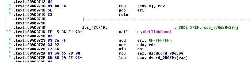
<p>To detour functions in the game we need to bypass an annoying <code class="language-plaintext highlighter-rouge">anti-debug</code>
feature introduced into the game that uses <code class="language-plaintext highlighter-rouge">GetTickCount</code> to analyse a thread’s
timing behaviour.</p>

<p>Using Cheat Engine I managed to trace the evil function to <code class="language-plaintext highlighter-rouge">0x004C06E0</code>:</p>

<div class="language-c highlighter-rouge"><div class="highlight"><pre class="highlight"><code><table class="rouge-table"><tbody><tr><td class="rouge-gutter gl"><pre class="lineno">1
</pre></td><td class="rouge-code"><pre><span class="cp">#define T5_Thread_Timer 0x004C06E0
</span></pre></td></tr></tbody></table></code></pre></div></div>

<p><img src="https://journal.lunar.sh/images/6/03.jpg" alt="Anti Debug Timer" />
Anti-debug timer view in <code class="language-plaintext highlighter-rouge">IDA</code>.</p>
<p>So make sure you patch this out otherwise the game will simply close after some
time after detouring.</p>

<p>We would have to hook the function before loading a solo zombie match as script
assets are loaded into memory shortly after starting a game mode. I wrote a
simple detouring library called <a href="https://github.com/lunar-sh/cdl86">cdl86</a>
that can <code class="language-plaintext highlighter-rouge">hook/detour</code> functions either by inserting a <code class="language-plaintext highlighter-rouge">JMP</code> opcode at the target
functions address to a detour function or through a software breakpoint.</p>

<p>I will leave this task up to the reader to perform. What you need is an address
and I took the liberty of finding the address of <code class="language-plaintext highlighter-rouge">DB_LinkXAssetEntry</code> for you in
<code class="language-plaintext highlighter-rouge">IDA Pro</code>. If you are wondering how I found the address, it would be a combination
of research, debugging and static analysis.</p>

<p>A lot comes down to recognising patterns in the disassembly. In general as you
find the address of functions it gradually becomes easier to find the address of
other related functions.</p>

<p>Bare in mind this is the address of the last <code class="language-plaintext highlighter-rouge">x86</code> (<code class="language-plaintext highlighter-rouge">32-bit</code>) <code class="language-plaintext highlighter-rouge">PC</code> version of the
game:</p>

<div class="language-c highlighter-rouge"><div class="highlight"><pre class="highlight"><code><table class="rouge-table"><tbody><tr><td class="rouge-gutter gl"><pre class="lineno">1
</pre></td><td class="rouge-code"><pre><span class="cp">#define T5_DB_LinkXAssetEntry 0x007A2F10
</span></pre></td></tr></tbody></table></code></pre></div></div>

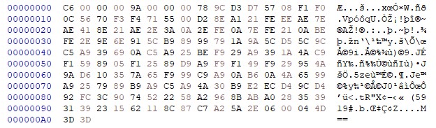
<p>Once you have a <code class="language-plaintext highlighter-rouge">GSC</code> script dump, open it in your favorite text editor (I used
<code class="language-plaintext highlighter-rouge">HxD</code>). This is a dump of a small <code class="language-plaintext highlighter-rouge">GSC</code> script from memory:</p>

<p><img src="https://journal.lunar.sh/images/6/02.jpg" alt="GSC Dump" /></p>

<p>We can immediately see that the script is not stored in simple plaintext. In
this case I like to look for <code class="language-plaintext highlighter-rouge">magic</code> bytes which may indicate if the file was
compressed. <code class="language-plaintext highlighter-rouge">zlib</code> compression is one of the most common compression types for
binary files.</p>

<p>Based off research I did, <code class="language-plaintext highlighter-rouge">zlib</code> uses the following magic bytes:</p>

<div class="language-plaintext highlighter-rouge"><div class="highlight"><pre class="highlight"><code><table class="rouge-table"><tbody><tr><td class="rouge-gutter gl"><pre class="lineno">1
2
3
</pre></td><td class="rouge-code"><pre>78 01 - No Compression/low
78 9C - Default Compression
78 DA - Best Compression
</pre></td></tr></tbody></table></code></pre></div></div>

<p>These bytes should appear not too far from the start of the file. Notice that in
the dump these bytes appear at offset <code class="language-plaintext highlighter-rouge">0x8</code> and <code class="language-plaintext highlighter-rouge">0x9</code> so there is a good chance
this file is <code class="language-plaintext highlighter-rouge">zlib</code> compressed. Let’s test this theory, here is a simple <code class="language-plaintext highlighter-rouge">zlib</code>
<code class="language-plaintext highlighter-rouge">inflate</code> python script:</p>

<div class="language-plaintext highlighter-rouge"><div class="highlight"><pre class="highlight"><code><table class="rouge-table"><tbody><tr><td class="rouge-gutter gl"><pre class="lineno">1
2
3
4
5
6
7
8
</pre></td><td class="rouge-code"><pre>import zlib

with open(sys.argv[1], 'rb') as compressed_data:
    compressed_data = compressed_data.read()
    unzipped = zlib.decompress(compressed_data[8:])
    with open(sys.argv[2], 'wb') as result:
        result.write(unzipped);
        result.close()
</pre></td></tr></tbody></table></code></pre></div></div>

<p>I get the following text:</p>

<div class="language-plaintext highlighter-rouge"><div class="highlight"><pre class="highlight"><code><table class="rouge-table"><tbody><tr><td class="rouge-gutter gl"><pre class="lineno">1
2
3
4
5
6
7
8
9
10
11
12
13
</pre></td><td class="rouge-code"><pre>// THIS FILE IS AUTOGENERATED, DO NOT MODIFY
main()
{
	self setModel("c_jap_takeo_body");
	self.voice = "vietnamese";
	self.skeleton = "base";
}

precache()
{
	precacheModel("c_jap_takeo_body");
}

</pre></td></tr></tbody></table></code></pre></div></div>
<p>This text has a size of <code class="language-plaintext highlighter-rouge">0xC6</code>.</p>

<p>Great and <code class="language-plaintext highlighter-rouge">+1</code> for the data being stored in plaintext!</p>

<p>So what are the first <code class="language-plaintext highlighter-rouge">8</code> bytes used for?</p>

<p>If you have a sharp eye you might have noticed that this 8 bytes actually
contains <code class="language-plaintext highlighter-rouge">2</code> values.</p>

<p>The first <code class="language-plaintext highlighter-rouge">4</code> bytes seems to represent our <code class="language-plaintext highlighter-rouge">inflated</code> (decompressed) data size of
<code class="language-plaintext highlighter-rouge">0xC6</code> and the second value seems to represent the <code class="language-plaintext highlighter-rouge">size of the file - 8 bytes</code>
or the size of our compressed data which is <code class="language-plaintext highlighter-rouge">0x9A</code>.</p>

<p>These values seem to be stored in <code class="language-plaintext highlighter-rouge">little-endian</code> format with the <code class="language-plaintext highlighter-rouge">4</code> byte integers
ordered as <code class="language-plaintext highlighter-rouge">LSB</code>.</p>

<p>Great we now have enough information to load a plaintext <code class="language-plaintext highlighter-rouge">GSC</code> script, compress it
and load it as an asset using <code class="language-plaintext highlighter-rouge">DB_LinkXAssetEntry</code>. It’s pretty cool that it is
this straightforward to decompress <code class="language-plaintext highlighter-rouge">GSC</code> scripts as it gives insight into how the
game modes/logic were implemented and plenty of ideas for mods of course!</p>

<p>So in theory we could inject a <code class="language-plaintext highlighter-rouge">DLL</code>, read our <code class="language-plaintext highlighter-rouge">GSC</code> script, compress it, link it
with <code class="language-plaintext highlighter-rouge">DB_LinkXAssetEntry</code> and then call <code class="language-plaintext highlighter-rouge">Scr_LoadScript</code> right? We will discuss
this in the next section.</p>

<h1 id="loading-and-executing-gsc-script-assets">Loading and executing GSC script assets</h1>

<p>It turns out that we cannot simply call <code class="language-plaintext highlighter-rouge">Scr_LoadScript</code> when we like. As
mentioned above <code class="language-plaintext highlighter-rouge">CoD</code> <code class="language-plaintext highlighter-rouge">Black Ops</code> will load all script assets using
<code class="language-plaintext highlighter-rouge">DB_LinkXAssetEntry</code> and then compile them using <code class="language-plaintext highlighter-rouge">Scr_LoadScript</code> while a map is
loading.</p>

<p>Therefore we have to load our <code class="language-plaintext highlighter-rouge">GSC</code> script at the correct time otherwise it won’t
work. The strategy is therefore to hook <code class="language-plaintext highlighter-rouge">Scr_LoadScript</code> and then load our
custom <code class="language-plaintext highlighter-rouge">GSC</code> script asset when <code class="language-plaintext highlighter-rouge">Scr_LoadScript</code> is loading one of the last <code class="language-plaintext highlighter-rouge">GSC</code>
scripts for the current map.</p>

<p>It turns out that one of the last <code class="language-plaintext highlighter-rouge">GSC</code> scripts contains the current map name.</p>

<p>To get the value of the current map we can utilize the function <code class="language-plaintext highlighter-rouge">Dvar_FindVar</code>
which i found to be at address: <code class="language-plaintext highlighter-rouge">0x0057FF80</code>:</p>

<div class="language-plaintext highlighter-rouge"><div class="highlight"><pre class="highlight"><code><table class="rouge-table"><tbody><tr><td class="rouge-gutter gl"><pre class="lineno">1
</pre></td><td class="rouge-code"><pre>#define T5_Dvar_FindVar 0x0057FF80
</pre></td></tr></tbody></table></code></pre></div></div>

<p>It’s function prototype is defined as follows:</p>
<div class="language-plaintext highlighter-rouge"><div class="highlight"><pre class="highlight"><code><table class="rouge-table"><tbody><tr><td class="rouge-gutter gl"><pre class="lineno">1
2
3
</pre></td><td class="rouge-code"><pre>typedef uint8_t* (__cdecl* Dvar_FindVar_t)(
	uint8_t* variable
);
</pre></td></tr></tbody></table></code></pre></div></div>

<p>The variable in question is <code class="language-plaintext highlighter-rouge">mapname</code> which will return the current map. It
should be noted that <code class="language-plaintext highlighter-rouge">Scr_LoadScript</code> does not execute our <code class="language-plaintext highlighter-rouge">GSC</code> script however,
instead we defer execution of our main function in our <code class="language-plaintext highlighter-rouge">GSC</code> script until the map
has finished loading.</p>

<p>To this end i found a convenient function that is called when the game is just
about to start at address <code class="language-plaintext highlighter-rouge">0x004B7F80</code>:</p>

<div class="language-plaintext highlighter-rouge"><div class="highlight"><pre class="highlight"><code><table class="rouge-table"><tbody><tr><td class="rouge-gutter gl"><pre class="lineno">1
</pre></td><td class="rouge-code"><pre>#define T5_Scr_LoadGameType 0x004B7F80
</pre></td></tr></tbody></table></code></pre></div></div>

<p>with the following signature:</p>
<div class="language-plaintext highlighter-rouge"><div class="highlight"><pre class="highlight"><code><table class="rouge-table"><tbody><tr><td class="rouge-gutter gl"><pre class="lineno">1
2
3
</pre></td><td class="rouge-code"><pre>typedef void (__cdecl* Scr_LoadGameType_t)(
	void
);
</pre></td></tr></tbody></table></code></pre></div></div>

<p>To defer execution however we need to obtain the function handle after the <code class="language-plaintext highlighter-rouge">GSC</code>
script has been loaded in our hooked <code class="language-plaintext highlighter-rouge">Scr_LoadScript</code>. In this case we utilize a
function called <code class="language-plaintext highlighter-rouge">Scr_GetFunctionHandle</code> which returns the address of a function
which has been loaded into the <code class="language-plaintext highlighter-rouge">GSC</code> execution environment or <code class="language-plaintext highlighter-rouge">VM</code>.</p>

<p>It has the following function signature:</p>

<div class="language-plaintext highlighter-rouge"><div class="highlight"><pre class="highlight"><code><table class="rouge-table"><tbody><tr><td class="rouge-gutter gl"><pre class="lineno">1
2
3
4
5
</pre></td><td class="rouge-code"><pre>typedef int32_t (__cdecl* Scr_GetFunctionHandle_t)(
	int32_t scriptInstance,
	const uint8_t* scriptName,
	const uint8_t* functioName
);
</pre></td></tr></tbody></table></code></pre></div></div>

<p><code class="language-plaintext highlighter-rouge">scriptInstance</code> is a variable which determines whether the script is a <code class="language-plaintext highlighter-rouge">GSC</code> or
<code class="language-plaintext highlighter-rouge">CSC</code> type script. A value of <code class="language-plaintext highlighter-rouge">0</code> indicates a <code class="language-plaintext highlighter-rouge">GSC</code> script while <code class="language-plaintext highlighter-rouge">1</code> indicated a <code class="language-plaintext highlighter-rouge">CSC</code>
script.</p>

<p>The function handle to our loaded script is then stored in a global variable and
the function can be executed in it’s own thread using <code class="language-plaintext highlighter-rouge">Scr_ExecThread</code> which has
the following prototype:</p>

<div class="language-plaintext highlighter-rouge"><div class="highlight"><pre class="highlight"><code><table class="rouge-table"><tbody><tr><td class="rouge-gutter gl"><pre class="lineno">1
2
3
4
5
</pre></td><td class="rouge-code"><pre>typedef uint16_t (__cdecl* Scr_ExecThread_t)(
	int32_t scriptInstance,
	int32_t handle,
	int32_t paramCount
);
</pre></td></tr></tbody></table></code></pre></div></div>

<p>I found this function at address: <code class="language-plaintext highlighter-rouge">0x005598E0</code>:</p>
<div class="language-plaintext highlighter-rouge"><div class="highlight"><pre class="highlight"><code><table class="rouge-table"><tbody><tr><td class="rouge-gutter gl"><pre class="lineno">1
</pre></td><td class="rouge-code"><pre>#define T5_Scr_ExecThread 0x005598E0
</pre></td></tr></tbody></table></code></pre></div></div>

<p>I also noticed during static analysis that a call to <code class="language-plaintext highlighter-rouge">T5_Scr_FreeThread</code> was
always made following a call to <code class="language-plaintext highlighter-rouge">Scr_ExecThread</code> so that the pseudo code would
look something like:</p>

<div class="language-plaintext highlighter-rouge"><div class="highlight"><pre class="highlight"><code><table class="rouge-table"><tbody><tr><td class="rouge-gutter gl"><pre class="lineno">1
2
</pre></td><td class="rouge-code"><pre>int16_t handle = Scr_ExecThread(0, func_handle, 0);
Scr_FreeThread(handle, 0);
</pre></td></tr></tbody></table></code></pre></div></div>

<p>We also obviously also need a compression library and for this I am using
<a href="https://github.com/lunar-sh/miniz">miniz</a>.</p>

<p>So to summarize the steps to inject our <code class="language-plaintext highlighter-rouge">GSC</code> script via our <code class="language-plaintext highlighter-rouge">Scr_LoadScript</code> hook:</p>

<ol>
  <li>Query map being loaded with <code class="language-plaintext highlighter-rouge">Dvar_FindVar</code>.</li>
  <li>Compare current <code class="language-plaintext highlighter-rouge">scriptName</code> with map name.</li>
  <li>On match open <code class="language-plaintext highlighter-rouge">GSC</code> script, compress and load asset as described above.</li>
  <li>Call <code class="language-plaintext highlighter-rouge">Scr_LoadScript</code> on our loaded script asset.</li>
  <li>Get function handle with <code class="language-plaintext highlighter-rouge">Scr_GetFunctionHandle</code>.</li>
</ol>

<p>To execute our <code class="language-plaintext highlighter-rouge">GSC</code> script entry function via our <code class="language-plaintext highlighter-rouge">Scr_LoadGameType_hk</code> hook:</p>
<ol>
  <li>Call <code class="language-plaintext highlighter-rouge">Scr_ExecThread</code> on function handle.</li>
  <li>Call <code class="language-plaintext highlighter-rouge">Scr_FreeThread</code> on handle returned by <code class="language-plaintext highlighter-rouge">Scr_ExecThread</code>.</li>
</ol>

<h1 id="black-ops-offsets">Black Ops Offsets</h1>

<p>I have included all the offsets I found for the game using <code class="language-plaintext highlighter-rouge">IDA</code>:</p>
<div class="language-plaintext highlighter-rouge"><div class="highlight"><pre class="highlight"><code><table class="rouge-table"><tbody><tr><td class="rouge-gutter gl"><pre class="lineno">1
2
3
4
5
6
7
8
9
10
</pre></td><td class="rouge-code"><pre>#define T5_Scr_LoadScript         0x00661AF0
#define T5_Scr_GetFunctionHandle  0x004E3470
#define T5_DB_LinkXAssetEntry     0x007A2F10
#define T5_Scr_ExecThread         0x005598E0
#define T5_Scr_FreeThread         0x005DE2C0
#define T5_Scr_LoadGameType       0x004B7F80
#define T5_Dvar_FindVar           0x0057FF80
#define T5_Assign_Hotfix          0x007A4800
#define T5_init_trigger           0x00C793B0
#define T5_Thread_Timer           0x004C06E0
</pre></td></tr></tbody></table></code></pre></div></div>

<p>A simple challenge would be to find these offsets yourself, it is not difficult.</p>

<p><code class="language-plaintext highlighter-rouge">Black Ops 1</code> uses the <code class="language-plaintext highlighter-rouge">__cdecl</code> calling convention for functions.</p>

<h1 id="source-code">Source Code</h1>

<p>I have included the source code of my simple <code class="language-plaintext highlighter-rouge">GSC</code> loader in the
<a href="https://github.com/lunar-sh/gsctool/">following</a> repo.</p>

<p>I have also included a sample <code class="language-plaintext highlighter-rouge">GSC</code> script that spawns a raygun at spawn in
zombies solo mode and dumps <code class="language-plaintext highlighter-rouge">GSC</code> scripts as they are loaded via a
<code class="language-plaintext highlighter-rouge">DB_LinkXAssetEntry</code> hook.</p>

<h1 id="demo">Demo</h1>

<p><img src="https://journal.lunar.sh/images/6/gscdemo.png" alt="" /></p>

<h1 id="signature">Signature</h1>

<div class="language-plaintext highlighter-rouge"><div class="highlight"><pre class="highlight"><code><table class="rouge-table"><tbody><tr><td class="rouge-gutter gl"><pre class="lineno">1
2
3
4
5
6
7
8
9
10
11
12
13
14
15
16
17
18
19
</pre></td><td class="rouge-code"><pre>+---------------------------------------+
|     .-.       .-.       .-.           |
|    /   \     /   \     /   \     +    |
|         \   /     \   /     \   /     |
|          "_"       "_"       "_"      |
|                                       |
|  _   _   _ _  _   _   ___   ___ _  _  |
| | | | | | | \| | /_\ | _ \ / __| || | |
| | |_| |_| | .` |/ _ \|   /_\__ \ __ | |
| |____\___/|_|\_/_/ \_\_|_(_)___/_||_| |
|                                       |
|                                       |
| Lunar RF Labs                         |
| Email: root@lunar.sh                  |
|                                       |
| Research Laboratories                 |
| OpenAlias (BTC, XMR): lunar.sh        |
| Copyright (C) 2022-2024               |
+---------------------------------------+
</pre></td></tr></tbody></table></code></pre></div></div>]]></content><author><name>Dylan Müller</name></author><summary type="html"><![CDATA[Learn how GSC scripts are loaded into Black Ops 1 and how to write your own simple GSC loader in C for the Microsoft Windows version of the game.]]></summary></entry><entry><title type="html">A Tiny C (x86_64) Function Hooking Library</title><link href="https://journal.lunar.sh/2022/linux-detours.html" rel="alternate" type="text/html" title="A Tiny C (x86_64) Function Hooking Library" /><published>2022-12-31T00:00:00+00:00</published><updated>2022-12-31T00:00:00+00:00</updated><id>https://journal.lunar.sh/2022/linux-detours</id><content type="html" xml:base="https://journal.lunar.sh/2022/linux-detours.html"><![CDATA[<blockquote>
  <p>Function detouring is a powerful hooking technique that allows for the
interception of <code class="language-plaintext highlighter-rouge">C/C++</code> functions. <code class="language-plaintext highlighter-rouge">cdl86</code> aims to be a tiny <code class="language-plaintext highlighter-rouge">C</code> detours
library for <code class="language-plaintext highlighter-rouge">x86_64</code> binaries.</p>
</blockquote>

<ol>
  <li><a href="#overview">Overview</a></li>
  <li><a href="#jmp-patching">JMP Patching</a></li>
  <li><a href="#int3-patching">INT3 Patching</a></li>
  <li><a href="#code-injection">Code Injection</a></li>
  <li><a href="#api">API</a></li>
  <li><a href="#source-code">Source Code</a></li>
</ol>

<h1 id="overview">Overview</h1>

<p>Note: This article details the linux specific details of the library. Windows
support has since been added.</p>

<p>See:
<a href="https://github.com/lunar-sh/cdl86">https://github.com/lunar-sh/cdl86</a></p>

<p><a href="https://en.wikipedia.org/wiki/Microsoft_Research">Microsoft Research</a> currently
maintains a library known as <a href="https://github.com/microsoft/Detours">MS Detours</a>.
It allows for the interception of Windows <code class="language-plaintext highlighter-rouge">API</code> calls within the memory address
space of a process.</p>

<p>This might be useful in certain situations such as if you are writing a <code class="language-plaintext highlighter-rouge">D3D9</code>
(<code class="language-plaintext highlighter-rouge">DirectX</code>) hook and you need to intercept cetain graphics routines. This is
commonly done for <code class="language-plaintext highlighter-rouge">ESP</code> and wallhacks where the <code class="language-plaintext highlighter-rouge">Z-buffer</code> needs to be
disabled for certain character models, for <code class="language-plaintext highlighter-rouge">D3D9</code> this might involve hooking
<code class="language-plaintext highlighter-rouge">DrawIndexedPrimitive</code>.</p>

<div class="language-plaintext highlighter-rouge"><div class="highlight"><pre class="highlight"><code><table class="rouge-table"><tbody><tr><td class="rouge-gutter gl"><pre class="lineno">1
2
3
4
5
6
7
8
9
10
</pre></td><td class="rouge-code"><pre>HRESULT WINAPI hkDrawIndexedPrimitive(LPDIRECT3DDEVICE9 pDevice, ...args)
{
    // Check play model strides, primitive count, etc
    ...
    pDevice-&gt;SetRenderState(D3DRS_ZENABLE, false);
    ...
    // Call original function and return
    oDrawIndexedPrimitive(...)
    return ...
}
</pre></td></tr></tbody></table></code></pre></div></div>

<p>In order to disable the <code class="language-plaintext highlighter-rouge">Z-buffer</code> in this example we need access to a valid
<code class="language-plaintext highlighter-rouge">LPDIRECT3DDEVICE9</code> context within the running process. This is where detours
comes in handy. Generally, the procedure to hook a specific function is as
follows:</p>

<ul>
  <li>Declare a function pointer with target function signature:</li>
</ul>

<div class="language-plaintext highlighter-rouge"><div class="highlight"><pre class="highlight"><code><table class="rouge-table"><tbody><tr><td class="rouge-gutter gl"><pre class="lineno">1
</pre></td><td class="rouge-code"><pre>typedef HRESULT (WINAPI* tDrawIndexedPrimitive)(LPDIRECT3DDEVICE9 pDevice, ...args);
</pre></td></tr></tbody></table></code></pre></div></div>

<ul>
  <li>Define detour function with same function signature:</li>
</ul>

<div class="language-plaintext highlighter-rouge"><div class="highlight"><pre class="highlight"><code><table class="rouge-table"><tbody><tr><td class="rouge-gutter gl"><pre class="lineno">1
</pre></td><td class="rouge-code"><pre>HRESULT WINAPI hkDrawIndexedPrimitive(LPDIRECT3DDEVICE9 pDevice, ...args)
</pre></td></tr></tbody></table></code></pre></div></div>

<ul>
  <li>Assign the function pointer the target functions address in memory. In this
case a <code class="language-plaintext highlighter-rouge">VTable</code> entry.</li>
</ul>

<div class="language-plaintext highlighter-rouge"><div class="highlight"><pre class="highlight"><code><table class="rouge-table"><tbody><tr><td class="rouge-gutter gl"><pre class="lineno">1
2
</pre></td><td class="rouge-code"><pre>#define DIP 0x55
tDrawIndexedPrimitive oDrawIndexedPrimitive = (oDrawIndexedPrimitive)SomeVTable[DIP];
</pre></td></tr></tbody></table></code></pre></div></div>

<ul>
  <li>Call DetourFunction:</li>
</ul>

<div class="language-plaintext highlighter-rouge"><div class="highlight"><pre class="highlight"><code><table class="rouge-table"><tbody><tr><td class="rouge-gutter gl"><pre class="lineno">1
</pre></td><td class="rouge-code"><pre>DetourFunction((void**)&amp;oDrawIndexedPrimitive, &amp;hkhkDrawIndexedPrimitive)
</pre></td></tr></tbody></table></code></pre></div></div>

<p><code class="language-plaintext highlighter-rouge">DetourFunction</code> then uses the <code class="language-plaintext highlighter-rouge">oDrawIndexedPrimitive</code> function pointer and
modifies the instructions at the target function in order to transfer control
flow to the detour function.</p>

<p>At this point any calls to <code class="language-plaintext highlighter-rouge">DrawIndexedPrimitive</code> within the <code class="language-plaintext highlighter-rouge">LPDIRECT3DDEVICE9</code>
class will be rerouted to <code class="language-plaintext highlighter-rouge">hkDrawIndexedPrimitive</code>. You can see that this is a
very powerful concept and gives us access to the callee’s function arguments. As
demonstrated, it is possible to hook both <code class="language-plaintext highlighter-rouge">C</code> and <code class="language-plaintext highlighter-rouge">C++</code> functions.</p>

<p>The difference generally is that the first argument to a <code class="language-plaintext highlighter-rouge">C++</code> function is a
hidden <code class="language-plaintext highlighter-rouge">this</code> pointer. Therefore you can define a <code class="language-plaintext highlighter-rouge">C++</code> detour in <code class="language-plaintext highlighter-rouge">C</code> with this
extra argument.</p>

<p>Detours is great, but it is only available for Windows. The aim of the <code class="language-plaintext highlighter-rouge">cdl86</code>
project is to create a simple, compact detours library for <code class="language-plaintext highlighter-rouge">x86_64</code> Linux. What
follows is a brief explanation on how the library was designed.</p>

<h1 id="detour-methods">Detour methods</h1>

<p>Two different approaches to method detouring were investigated and implemented
in the <code class="language-plaintext highlighter-rouge">cdl86</code> <code class="language-plaintext highlighter-rouge">C</code> library. First let’s have a look at a typical function call for a
simple <code class="language-plaintext highlighter-rouge">C</code> program. We will be using <code class="language-plaintext highlighter-rouge">GDB</code> to inspect the resulting disassembly.</p>

<div class="language-plaintext highlighter-rouge"><div class="highlight"><pre class="highlight"><code><table class="rouge-table"><tbody><tr><td class="rouge-gutter gl"><pre class="lineno">1
2
3
4
5
6
7
8
9
10
11
</pre></td><td class="rouge-code"><pre>#include &lt;stdio.h&gt;

int add(int x, int y)
{
    return x + y;
}
int main()
{
    printf("%i", add(1,1));
    return 0;
}
</pre></td></tr></tbody></table></code></pre></div></div>

<p>Compile with:</p>
<div class="language-plaintext highlighter-rouge"><div class="highlight"><pre class="highlight"><code><table class="rouge-table"><tbody><tr><td class="rouge-gutter gl"><pre class="lineno">1
</pre></td><td class="rouge-code"><pre>gcc main.c -o main
</pre></td></tr></tbody></table></code></pre></div></div>

<p>and then debug with <code class="language-plaintext highlighter-rouge">GDB</code>:</p>

<div class="language-plaintext highlighter-rouge"><div class="highlight"><pre class="highlight"><code><table class="rouge-table"><tbody><tr><td class="rouge-gutter gl"><pre class="lineno">1
</pre></td><td class="rouge-code"><pre>gdb main
</pre></td></tr></tbody></table></code></pre></div></div>

<p>To list all the functions in the binary, supply <code class="language-plaintext highlighter-rouge">info functions</code> to the <code class="language-plaintext highlighter-rouge">gdb</code>
command prompt.</p>

<div class="language-plaintext highlighter-rouge"><div class="highlight"><pre class="highlight"><code><table class="rouge-table"><tbody><tr><td class="rouge-gutter gl"><pre class="lineno">1
2
3
4
5
6
7
</pre></td><td class="rouge-code"><pre>0x0000000000001100  __do_global_dtors_aux
0x0000000000001140  frame_dummy
0x0000000000001149  add
0x0000000000001161  main
0x00000000000011a0  __libc_csu_init
0x0000000000001210  __libc_csu_fini
0x0000000000001218  _fini
</pre></td></tr></tbody></table></code></pre></div></div>

<p>Let’s disassemble the main function with <code class="language-plaintext highlighter-rouge">disas /r main</code>:</p>

<div class="language-plaintext highlighter-rouge"><div class="highlight"><pre class="highlight"><code><table class="rouge-table"><tbody><tr><td class="rouge-gutter gl"><pre class="lineno">1
2
3
4
5
6
7
8
</pre></td><td class="rouge-code"><pre>Dump of assembler code for function main:
   0x0000000000001161 &lt;+0&gt;:     f3 0f 1e fa     endbr64
   0x0000000000001165 &lt;+4&gt;:     55      push   %rbp
   0x0000000000001166 &lt;+5&gt;:     48 89 e5        mov    %rsp,%rbp
   0x0000000000001169 &lt;+8&gt;:     be 01 00 00 00  mov    $0x1,%esi
   0x000000000000116e &lt;+13&gt;:    bf 01 00 00 00  mov    $0x1,%edi
   0x0000000000001173 &lt;+18&gt;:    e8 d1 ff ff ff  callq  0x1149 &lt;add&gt;
   0x0000000000001178 &lt;+23&gt;:    89 c6   mov    %eax,%esi
</pre></td></tr></tbody></table></code></pre></div></div>

<p><code class="language-plaintext highlighter-rouge">callq</code> has one operand which is the address of the function being called. It
pushes the current value of <code class="language-plaintext highlighter-rouge">%rip</code> (next instruction after call) onto the stack
and then transfers control flow to the target function.</p>

<p>You may have also noticed the presence of the <code class="language-plaintext highlighter-rouge">endbr64</code> instruction. This
instruction is specific to Intel processors and is part of <a href="https://software.intel.com/content/www/us/en/develop/articles/technical-look-control-flow-enforcement-technology.html">Intel’s Control-Flow
Enforcement Technology
(CET)</a>.
<code class="language-plaintext highlighter-rouge">CET</code> is designed to provide hardware protection against <code class="language-plaintext highlighter-rouge">ROP</code> (Return-orientated
Programming) and similar methods which manipulate control flow using <em>existing</em>
byte code.</p>

<p>It’s two main features are:</p>

<ul>
  <li>A shadow stack for tracking return addresses.</li>
  <li>Indirect branch tracking, which <code class="language-plaintext highlighter-rouge">endbr64</code> is a part of.</li>
</ul>

<p><code class="language-plaintext highlighter-rouge">Intel CET</code> however does not prevent us from modifying control flow <strong>directly</strong>
by inserting instructions into memory.</p>

<h1 id="jmp-patching">JMP Patching</h1>

<p>The first method of function detouring we will explore is by inserting a <code class="language-plaintext highlighter-rouge">JMP</code>
instruction at the beginning of the target function to transfer control over to
the detour function. It should be noted that in order to preserve the stack we
need to use a <code class="language-plaintext highlighter-rouge">JMP</code> (specifically <code class="language-plaintext highlighter-rouge">jmpq</code>) instruction rather than a <code class="language-plaintext highlighter-rouge">CALL</code>.</p>

<p>Since there is no way to pass a <code class="language-plaintext highlighter-rouge">64-bit</code> address to the <code class="language-plaintext highlighter-rouge">jmpq</code> instruction we will
have to first store the address we want to jump to into a register. We need to
choose a register that is not part of the <code class="language-plaintext highlighter-rouge">__cdecl</code> (defualt) calling
convention. <code class="language-plaintext highlighter-rouge">%rax</code> happens to be a register that is not part of the <code class="language-plaintext highlighter-rouge">__cdecl</code>
userspace calling convention and so for simplicity we use this register in our
design.</p>

<p>The following is a disassembly of the instructions required for a <code class="language-plaintext highlighter-rouge">JMP</code> to a
<code class="language-plaintext highlighter-rouge">64-bit</code> immediate address:</p>

<div class="language-plaintext highlighter-rouge"><div class="highlight"><pre class="highlight"><code><table class="rouge-table"><tbody><tr><td class="rouge-gutter gl"><pre class="lineno">1
2
</pre></td><td class="rouge-code"><pre>0x0000555555561389 &lt;+0&gt;: 48 b8 b1 13 56 55 55 55 00 00 movabs $0x5555555613b1,%rax
0x0000555555561393 &lt;+10&gt;: ff e0	jmpq   *%rax
</pre></td></tr></tbody></table></code></pre></div></div>

<p>You can see that <code class="language-plaintext highlighter-rouge">12</code> bytes are required to encode the <code class="language-plaintext highlighter-rouge">movabs</code> instruction (which
moves the detour address into <code class="language-plaintext highlighter-rouge">%rax</code>) as well as the <code class="language-plaintext highlighter-rouge">jmpq</code> instruction.
Immediate values are stored in little endian (LE) encoding.</p>

<p>So we can therefore conclude that we need to patch <strong>at least</strong> <code class="language-plaintext highlighter-rouge">12</code> bytes in
memory at the location of our target function. These <code class="language-plaintext highlighter-rouge">12</code> bytes however are
important and we cannot simply discard them. It turns out that we actually place
these bytes at the start of what I will call a ‘trampoline function’, it’s
layout is as follows:</p>

<div class="language-plaintext highlighter-rouge"><div class="highlight"><pre class="highlight"><code><table class="rouge-table"><tbody><tr><td class="rouge-gutter gl"><pre class="lineno">1
2
3
</pre></td><td class="rouge-code"><pre>trampoline &lt;0x23215412&gt;:
    (original instruction bytes which were patched)
    JMP (target + JMP patch length)
</pre></td></tr></tbody></table></code></pre></div></div>

<p>Simply put, the trampoline function behaves as the original, unpatched function.
As shown above it consists of the target function’s original instruction bytes
as well as a call to the target function, offset by the <code class="language-plaintext highlighter-rouge">JMP</code> patch length.</p>

<p>The trampoline generation code for <code class="language-plaintext highlighter-rouge">cdl86</code> is shown below:</p>

<div class="language-plaintext highlighter-rouge"><div class="highlight"><pre class="highlight"><code><table class="rouge-table"><tbody><tr><td class="rouge-gutter gl"><pre class="lineno">1
2
3
4
5
6
7
8
9
10
11
12
13
14
15
16
17
18
19
20
21
</pre></td><td class="rouge-code"><pre>uint8_t *cdl_gen_trampoline(uint8_t *target, uint8_t *bytes_orig, int size)
{
    uint8_t *trampoline;
    int prot = 0x0;
    int flags = 0x0;

    /* New function should have read, write and
     * execute permissions.
     */
    prot = PROT_READ | PROT_WRITE | PROT_EXEC;
    flags = MAP_PRIVATE | MAP_ANONYMOUS;

    /* We use mmap to allocate trampoline memory pool. */
    trampoline = mmap(NULL, size + BYTES_JMP_PATCH, prot, flags, -1, 0);
    memcpy(trampoline, bytes_orig, size);
    /* Generate jump to address just after call
     * to detour in trampoline. */
    cdl_gen_jmpq_rax(trampoline + size, target + size);

    return trampoline;
}
</pre></td></tr></tbody></table></code></pre></div></div>

<p>You can see that the allocation of the trampoline function occurs through a call
to <code class="language-plaintext highlighter-rouge">mmap</code> with the <code class="language-plaintext highlighter-rouge">PROT_READ | PROT_WRITE | PROT_EXEC</code> memory protection flags.</p>

<p>Therefore it should also be noted that the correct memory permissions should be
set for both the target function before modification as well as the trampoline
function, after allocation. Here is a snippet from the <code class="language-plaintext highlighter-rouge">cdl86</code> library for
setting memory attributes:</p>

<div class="language-plaintext highlighter-rouge"><div class="highlight"><pre class="highlight"><code><table class="rouge-table"><tbody><tr><td class="rouge-gutter gl"><pre class="lineno">1
2
3
4
5
6
7
8
9
10
11
12
13
14
</pre></td><td class="rouge-code"><pre>/* Set R/W memory protections for code page. */
int cdl_set_page_protect(uint8_t *code)
{
    int perms = 0x0;
    int ret = 0x0;

    /* Read, write and execute perms. */
    perms = PROT_EXEC | PROT_READ | PROT_WRITE;
    /* Calculate page size */
    uintptr_t page_size = sysconf(_SC_PAGE_SIZE);
    ret = mprotect(code - ((uintptr_t)(code) % page_size), page_size, perms);

    return ret;
}
</pre></td></tr></tbody></table></code></pre></div></div>

<p>The general procedure to place the <code class="language-plaintext highlighter-rouge">JMP</code> hook is as follows:</p>

<ol>
  <li>Determine the minimum number of bytes required for a <code class="language-plaintext highlighter-rouge">JMP</code> patch.</li>
  <li>Create trampoline function.</li>
  <li>Set memory permissions (read, write, execute).</li>
  <li>Generate <code class="language-plaintext highlighter-rouge">JMP</code> to detour at target function.</li>
  <li>Fill unused bytes with <code class="language-plaintext highlighter-rouge">NOP</code>.</li>
  <li>Assign trampoline address to target function pointer.</li>
</ol>

<p>Let’s have a look at all of this in action using <code class="language-plaintext highlighter-rouge">GDB</code>. I will be using the
<a href="https://github.com/lunar-sh/cdl86/blob/master/tests/basic_jmp.c">basic_jmp.c</a>
test case in the <code class="language-plaintext highlighter-rouge">cdl86</code> library. The source code for this test case is shown
below:</p>

<div class="language-plaintext highlighter-rouge"><div class="highlight"><pre class="highlight"><code><table class="rouge-table"><tbody><tr><td class="rouge-gutter gl"><pre class="lineno">1
2
3
4
5
6
7
8
9
10
11
12
13
14
15
16
17
18
19
20
21
22
23
24
25
26
27
28
29
30
31
32
33
34
35
36
37
38
39
40
</pre></td><td class="rouge-code"><pre>#include "cdl.h"

typedef int add_t(int x, int y);
add_t *addo = NULL;

int add(int x, int y)
{
    printf("Inside original function\n");
    return x + y;
}

int add_detour(int x, int y)
{
    printf("Inside detour function\n");
    return addo(5,5);
}

int main()
{
    struct cdl_jmp_patch jmp_patch = {};
    addo = (add_t*)add;

    printf("Before attach: \n");
    printf("add(1,1) = %i\n\n", add(1,1));

    jmp_patch = cdl_jmp_attach((void**)&amp;addo, add_detour);
    if(jmp_patch.active)
    {
        printf("After attach: \n");
        printf("add(1,1) = %i\n\n", add(1,1));
        printf("== DEBUG INFO ==\n");
        cdl_jmp_dbg(&amp;jmp_patch);
    }

    cdl_jmp_detach(&amp;jmp_patch);
    printf("\nAfter detach: \n");
    printf("add(1,1) = %i\n\n", add(1,1));

    return 0;
}
</pre></td></tr></tbody></table></code></pre></div></div>

<p>We compile the following source file with (modified from makefile):</p>

<div class="language-plaintext highlighter-rouge"><div class="highlight"><pre class="highlight"><code><table class="rouge-table"><tbody><tr><td class="rouge-gutter gl"><pre class="lineno">1
</pre></td><td class="rouge-code"><pre>gcc -I../ -g basic_jmp.c ../cdl.c ../lib/libudis86/*.c -g -o basic_jmp
</pre></td></tr></tbody></table></code></pre></div></div>

<p>Then load into <code class="language-plaintext highlighter-rouge">GDB</code> using:</p>

<div class="language-plaintext highlighter-rouge"><div class="highlight"><pre class="highlight"><code><table class="rouge-table"><tbody><tr><td class="rouge-gutter gl"><pre class="lineno">1
</pre></td><td class="rouge-code"><pre>gdb basic_jmp
</pre></td></tr></tbody></table></code></pre></div></div>

<p>Once <code class="language-plaintext highlighter-rouge">GDB</code> has loaded, we insert a breakpoints at lines <code class="language-plaintext highlighter-rouge">24</code> and <code class="language-plaintext highlighter-rouge">27</code> using the
command:</p>

<div class="language-plaintext highlighter-rouge"><div class="highlight"><pre class="highlight"><code><table class="rouge-table"><tbody><tr><td class="rouge-gutter gl"><pre class="lineno">1
2
</pre></td><td class="rouge-code"><pre>break 24
break 27
</pre></td></tr></tbody></table></code></pre></div></div>

<p>We start execution of the program with:</p>

<div class="language-plaintext highlighter-rouge"><div class="highlight"><pre class="highlight"><code><table class="rouge-table"><tbody><tr><td class="rouge-gutter gl"><pre class="lineno">1
</pre></td><td class="rouge-code"><pre>run
</pre></td></tr></tbody></table></code></pre></div></div>

<p><code class="language-plaintext highlighter-rouge">GDB</code> will then inform you that the first breakpoint has been triggered. For this
first breakpoint we are interested in the <code class="language-plaintext highlighter-rouge">add()</code> function’s assembly before the
hook has taken place. To inspect this assembly, provide:</p>

<div class="language-plaintext highlighter-rouge"><div class="highlight"><pre class="highlight"><code><table class="rouge-table"><tbody><tr><td class="rouge-gutter gl"><pre class="lineno">1
</pre></td><td class="rouge-code"><pre>disas /r add
</pre></td></tr></tbody></table></code></pre></div></div>
<div class="language-plaintext highlighter-rouge"><div class="highlight"><pre class="highlight"><code><table class="rouge-table"><tbody><tr><td class="rouge-gutter gl"><pre class="lineno">1
2
3
4
5
6
</pre></td><td class="rouge-code"><pre>Dump of assembler code for function add:
   0x0000555555561389 &lt;+0&gt;:	f3 0f 1e fa	endbr64
   0x000055555556138d &lt;+4&gt;:	55	push   %rbp
   0x000055555556138e &lt;+5&gt;:	48 89 e5	mov    %rsp,%rbp
   0x0000555555561391 &lt;+8&gt;:	48 83 ec 10	sub    $0x10,%rsp
   0x0000555555561395 &lt;+12&gt;:	89 7d fc	mov    %edi,-0x4(%rbp)
</pre></td></tr></tbody></table></code></pre></div></div>

<p>This is the disassembly of the unaltered target function. <code class="language-plaintext highlighter-rouge">12</code> bytes for the <code class="language-plaintext highlighter-rouge">JMP</code>
patch will have to be written at this address. Therefore the first <code class="language-plaintext highlighter-rouge">4</code>
instructions will need to be written to the trampoline function followed by a
<code class="language-plaintext highlighter-rouge">JMP</code> to address <code class="language-plaintext highlighter-rouge">0x0000555555561395</code> and that’s all we need for the trampoline!</p>

<p>Now the fun part! Let’s continue execution to the next breakpoint, where our
<code class="language-plaintext highlighter-rouge">JMP</code> hook will be placed.</p>

<div class="language-plaintext highlighter-rouge"><div class="highlight"><pre class="highlight"><code><table class="rouge-table"><tbody><tr><td class="rouge-gutter gl"><pre class="lineno">1
</pre></td><td class="rouge-code"><pre>continue
</pre></td></tr></tbody></table></code></pre></div></div>

<p>Let’s examine the disassembly of our <code class="language-plaintext highlighter-rouge">add()</code> function once again:</p>

<div class="language-plaintext highlighter-rouge"><div class="highlight"><pre class="highlight"><code><table class="rouge-table"><tbody><tr><td class="rouge-gutter gl"><pre class="lineno">1
2
3
4
5
</pre></td><td class="rouge-code"><pre>Dump of assembler code for function add:
   0x0000555555561389 &lt;+0&gt;: 48 b8 b1 13 56 55 55 55 00 00 movabs $0x5555555613b1,%rax
   0x0000555555561393 &lt;+10&gt;: ff e0	jmpq   *%rax
   0x0000555555561395 &lt;+12&gt;: 89 7d fc	mov    %edi,-0x4(%rbp)
   0x0000555555561398 &lt;+15&gt;: 89 75 f8	mov    %esi,-0x8(%rbp)
</pre></td></tr></tbody></table></code></pre></div></div>

<p><code class="language-plaintext highlighter-rouge">0x5555555613b1</code> is the address of our detour/intercept function. Let’s examine
the disassembly of our detour function:</p>

<div class="language-plaintext highlighter-rouge"><div class="highlight"><pre class="highlight"><code><table class="rouge-table"><tbody><tr><td class="rouge-gutter gl"><pre class="lineno">1
</pre></td><td class="rouge-code"><pre>disas /r 0x5555555613b1
</pre></td></tr></tbody></table></code></pre></div></div>

<div class="language-plaintext highlighter-rouge"><div class="highlight"><pre class="highlight"><code><table class="rouge-table"><tbody><tr><td class="rouge-gutter gl"><pre class="lineno">1
2
3
4
5
6
7
8
9
10
11
12
13
14
15
</pre></td><td class="rouge-code"><pre>Dump of assembler code for function add_detour:
   0x00005555555613b1 &lt;+0&gt;:	f3 0f 1e fa	endbr64
   0x00005555555613b5 &lt;+4&gt;:	55	push   %rbp
   0x00005555555613b6 &lt;+5&gt;:	48 89 e5	mov    %rsp,%rbp
   0x00005555555613b9 &lt;+8&gt;:	48 83 ec 10	sub    $0x10,%rsp
   0x00005555555613bd &lt;+12&gt;:	89 7d fc	mov    %edi,-0x4(%rbp)
   0x00005555555613c0 &lt;+15&gt;:	89 75 f8	mov    %esi,-0x8(%rbp)
   0x00005555555613c3 &lt;+18&gt;:	48 8d 3d 53 5c 00 00	lea    0x5c53(%rip),%rdi
   0x00005555555613ca &lt;+25&gt;:	e8 b1 fd ff ff	callq  0x555555561180 &lt;puts@plt&gt;
   0x00005555555613cf &lt;+30&gt;:	48 8b 05 ba bc 01 00	mov    0x1bcba(%rip),%rax
   0x00005555555613d6 &lt;+37&gt;:	be 05 00 00 00	mov    $0x5,%esi
   0x00005555555613db &lt;+42&gt;:	bf 05 00 00 00	mov    $0x5,%edi
   0x00005555555613e0 &lt;+47&gt;:	ff d0	callq  *%rax
   0x00005555555613e2 &lt;+49&gt;:	c9	leaveq
   0x00005555555613e3 &lt;+50&gt;:	c3	retq
</pre></td></tr></tbody></table></code></pre></div></div>

<p>We can see that a call to our trampoline function is made to the address given
by referencing the <code class="language-plaintext highlighter-rouge">QWORD</code> (out function pointer) at address <code class="language-plaintext highlighter-rouge">0x55555557d090</code>,
let’s deference it:</p>

<div class="language-plaintext highlighter-rouge"><div class="highlight"><pre class="highlight"><code><table class="rouge-table"><tbody><tr><td class="rouge-gutter gl"><pre class="lineno">1
</pre></td><td class="rouge-code"><pre>print /x *(long unsigned int*)(0x55555557d090)
</pre></td></tr></tbody></table></code></pre></div></div>
<div class="language-plaintext highlighter-rouge"><div class="highlight"><pre class="highlight"><code><table class="rouge-table"><tbody><tr><td class="rouge-gutter gl"><pre class="lineno">1
</pre></td><td class="rouge-code"><pre>$20 = 0x7ffff7ffb000
</pre></td></tr></tbody></table></code></pre></div></div>

<p>So the function pointer is pointing to address <code class="language-plaintext highlighter-rouge">0x7ffff7ffb000</code> which is our
trampoline function, let’s dissasemble it:</p>

<div class="language-plaintext highlighter-rouge"><div class="highlight"><pre class="highlight"><code><table class="rouge-table"><tbody><tr><td class="rouge-gutter gl"><pre class="lineno">1
</pre></td><td class="rouge-code"><pre>x/10i 0x7ffff7ffb000
</pre></td></tr></tbody></table></code></pre></div></div>

<div class="language-plaintext highlighter-rouge"><div class="highlight"><pre class="highlight"><code><table class="rouge-table"><tbody><tr><td class="rouge-gutter gl"><pre class="lineno">1
2
3
4
5
6
7
8
9
10
</pre></td><td class="rouge-code"><pre>   0x7ffff7ffb000:	endbr64
   0x7ffff7ffb004:	push   %rbp
   0x7ffff7ffb005:	mov    %rsp,%rbp
   0x7ffff7ffb008:	sub    $0x10,%rsp
   0x7ffff7ffb00c:	movabs $0x555555561395,%rax
   0x7ffff7ffb016:	jmpq   *%rax
   0x7ffff7ffb018:	add    %al,(%rax)
   0x7ffff7ffb01a:	add    %al,(%rax)
   0x7ffff7ffb01c:	add    %al,(%rax)
   0x7ffff7ffb01e:	add    %al,(%rax)
</pre></td></tr></tbody></table></code></pre></div></div>

<p>You can see that our trampoline contains the first <code class="language-plaintext highlighter-rouge">4</code> instructions that were
replaced when the <code class="language-plaintext highlighter-rouge">JMP</code> patch was placed in our target function. You can see a
jmp back to address <code class="language-plaintext highlighter-rouge">0x555555561395</code> which was disassembled earlier. This should
give you an idea of how the control flow modification is achieved.</p>

<h1 id="int3-patching">INT3 Patching</h1>

<p>There is another method of function detouring which involves placing <code class="language-plaintext highlighter-rouge">INT3</code>
breakpoints at the start of the target function in memory. <code class="language-plaintext highlighter-rouge">INT3</code> breakpoints
are encoded with the <code class="language-plaintext highlighter-rouge">0xCC</code> opcode:</p>

<div class="language-plaintext highlighter-rouge"><div class="highlight"><pre class="highlight"><code><table class="rouge-table"><tbody><tr><td class="rouge-gutter gl"><pre class="lineno">1
2
3
4
5
6
</pre></td><td class="rouge-code"><pre>/* Generate int3 instruction. */
uint8_t *cdl_gen_swbp(uint8_t *code)
{
    *(code + 0x0) = 0xCC;
    return code;
}
</pre></td></tr></tbody></table></code></pre></div></div>

<p>So rather than placing a <code class="language-plaintext highlighter-rouge">JMP</code> patch to the detour we simply write the byte
<code class="language-plaintext highlighter-rouge">0xCC</code> to the target function being careful to <code class="language-plaintext highlighter-rouge">NOP</code> the unused bytes. Once the
<code class="language-plaintext highlighter-rouge">RIP</code> register reaches an address of an <code class="language-plaintext highlighter-rouge">INT3</code> breakpoint the Linux kernel sends
a <code class="language-plaintext highlighter-rouge">SIGTRAP</code> signal to the process.</p>

<p>We can register our own signal handler but we need some additional info on the
signal such as context information. A context is the state of a program’s
registers and stack. We need this info to compare the breakpoints <code class="language-plaintext highlighter-rouge">RIP</code> value to
any active global software breakpoints.</p>

<p>This is how the signal handler is registered in <code class="language-plaintext highlighter-rouge">cdl86</code>:</p>

<div class="language-plaintext highlighter-rouge"><div class="highlight"><pre class="highlight"><code><table class="rouge-table"><tbody><tr><td class="rouge-gutter gl"><pre class="lineno">1
2
3
4
5
6
7
8
9
10
11
12
13
14
</pre></td><td class="rouge-code"><pre> struct sigaction sa = {};

    /* Initialise cdl signal handler. */
    if (!cdl_swbp_init)
    {
        /* Request signal context info which
         * is required for RIP register comparison.
         */
        sa.sa_flags = SA_SIGINFO | SA_ONESHOT;
        sa.sa_sigaction = (void *)cdl_swbp_handler;
        sigaction(SIGTRAP, &amp;sa, NULL);
        cdl_swbp_init = true;
    }
    ...
</pre></td></tr></tbody></table></code></pre></div></div>

<p>Note the use of <code class="language-plaintext highlighter-rouge">SA_SIGINFO</code> to get context information. The software breakpoint
handler is then defined as follows:</p>

<div class="language-plaintext highlighter-rouge"><div class="highlight"><pre class="highlight"><code><table class="rouge-table"><tbody><tr><td class="rouge-gutter gl"><pre class="lineno">1
2
3
4
5
6
7
8
9
10
11
12
13
14
15
16
17
18
19
20
21
22
23
24
</pre></td><td class="rouge-code"><pre>void cdl_swbp_handler(int sig, siginfo_t *info, struct ucontext_t *context)
{
    int i = 0x0;
    bool active = false;
    uint8_t *bp_addr = NULL;

    /* RIP register point to instruction after the
     * int3 breakpoint so we subtract 0x1.
     */
    bp_addr = (uint8_t *)(context-&gt;uc_mcontext.gregs[REG_RIP] - 0x1);

    /* Iterate over all breakpoint structs. */
    for (i = 0; i &lt; cdl_swbp_size; i++)
    {
        active = cdl_swbp_hk[i].active;
        /* Compare breakpoint addresses. */
        if (bp_addr == cdl_swbp_hk[i].bp_addr)
        {
            /* Update RIP and reset context. */
            context-&gt;uc_mcontext.gregs[REG_RIP] = (greg_t)cdl_swbp_hk[i].detour;
            setcontext(context);
        }
    }
}
</pre></td></tr></tbody></table></code></pre></div></div>

<p>Note that if a match of the <code class="language-plaintext highlighter-rouge">RIP</code> value to any known breakpoints occurs the <code class="language-plaintext highlighter-rouge">RIP</code>
value for the current context is updated and the new context applied using
<code class="language-plaintext highlighter-rouge">setcontext()</code>. A trampoline function similar to our <code class="language-plaintext highlighter-rouge">JMP</code> patch is allocated
and serves the same purpose.</p>

<h1 id="code-injection">Code Injection</h1>

<p><code class="language-plaintext highlighter-rouge">cdl86</code> assumes that you are operating in the address space of the target
process. Therefore code injection is often required in practice and requires the
use of an
<a href="https://github.com/lunar-sh/robocraft/tree/main/injector">injector</a>.</p>

<p>Once a shared library (<code class="language-plaintext highlighter-rouge">.so</code>) has been injected you can use the following code
to get the base address of the main executable module:</p>

<div class="language-plaintext highlighter-rouge"><div class="highlight"><pre class="highlight"><code><table class="rouge-table"><tbody><tr><td class="rouge-gutter gl"><pre class="lineno">1
2
3
4
5
6
7
8
9
10
11
</pre></td><td class="rouge-code"><pre>#include &lt;link.h&gt;
#include &lt;inttypes.h&gt;

int __attribute__((constructor)) init()
{
...
    struct link_map *lm = dlopen(0, RTLD_NOW);
    printf("base = %" PRIx64 , lm-&gt;l_addr);
...

}
</pre></td></tr></tbody></table></code></pre></div></div>

<p>Or find the address of a function by symbol name:</p>

<div class="language-plaintext highlighter-rouge"><div class="highlight"><pre class="highlight"><code><table class="rouge-table"><tbody><tr><td class="rouge-gutter gl"><pre class="lineno">1
2
</pre></td><td class="rouge-code"><pre>void* dl_handle = dlopen(NULL, RTLD_LAZY);
void* add_ptr = dlsym(dl_handle, "add");
</pre></td></tr></tbody></table></code></pre></div></div>

<h1 id="api">API</h1>
<p>The API for the <code class="language-plaintext highlighter-rouge">cdl86</code> library is shown below:</p>

<div class="language-plaintext highlighter-rouge"><div class="highlight"><pre class="highlight"><code><table class="rouge-table"><tbody><tr><td class="rouge-gutter gl"><pre class="lineno">1
2
3
4
5
6
</pre></td><td class="rouge-code"><pre>struct cdl_jmp_patch cdl_jmp_attach(void **target, void *detour);
struct cdl_swbp_patch cdl_swbp_attach(void **target, void *detour);
void cdl_jmp_detach(struct cdl_jmp_patch *jmp_patch);
void cdl_swbp_detach(struct cdl_swbp_patch *swbp_patch);
void cdl_jmp_dbg(struct cdl_jmp_patch *jmp_patch);
void cdl_swbp_dbg(struct cdl_swbp_patch *swbp_patch);
</pre></td></tr></tbody></table></code></pre></div></div>

<h1 id="source-code">Source code</h1>
<p>You can find the <code class="language-plaintext highlighter-rouge">cdl86</code> source code
<a href="https://github.com/lunar-sh/cdl86">here</a>.<br /></p>

<h1 id="signature">Signature</h1>

<div class="language-plaintext highlighter-rouge"><div class="highlight"><pre class="highlight"><code><table class="rouge-table"><tbody><tr><td class="rouge-gutter gl"><pre class="lineno">1
2
3
4
5
6
7
8
9
10
11
12
13
14
15
16
17
18
19
</pre></td><td class="rouge-code"><pre>+---------------------------------------+
|     .-.       .-.       .-.           |
|    /   \     /   \     /   \     +    |
|         \   /     \   /     \   /     |
|          "_"       "_"       "_"      |
|                                       |
|  _   _   _ _  _   _   ___   ___ _  _  |
| | | | | | | \| | /_\ | _ \ / __| || | |
| | |_| |_| | .` |/ _ \|   /_\__ \ __ | |
| |____\___/|_|\_/_/ \_\_|_(_)___/_||_| |
|                                       |
|                                       |
| Lunar RF Labs                         |
| Email: root@lunar.sh                  |
|                                       |
| Research Laboratories                 |
| OpenAlias (BTC, XMR): lunar.sh        |
| Copyright (C) 2022-2024               |
+---------------------------------------+
</pre></td></tr></tbody></table></code></pre></div></div>]]></content><author><name>Dylan Müller</name></author><summary type="html"><![CDATA[Function detouring is a powerful hooking technique that allows for the interception of C/C++ functions. cdl86 aims to be a tiny C detours library for x86_64 binaries.]]></summary></entry><entry><title type="html">Mono/.NET Injection Under Linux</title><link href="https://journal.lunar.sh/2020/mono-dot-net-injection.html" rel="alternate" type="text/html" title="Mono/.NET Injection Under Linux" /><published>2020-12-11T00:00:00+00:00</published><updated>2020-12-11T00:00:00+00:00</updated><id>https://journal.lunar.sh/2020/mono-dot-net-injection</id><content type="html" xml:base="https://journal.lunar.sh/2020/mono-dot-net-injection.html"><![CDATA[<blockquote>
  <p>Learning <code class="language-plaintext highlighter-rouge">mono</code> or <code class="language-plaintext highlighter-rouge">C#</code> library injection through a Robocraft exploit. The method used in
this publication can be used to modify a wide range of Unity games.</p>
</blockquote>

<ol>
  <li><a href="#mono-overview">Mono Overview</a></li>
  <li><a href="#exploiting-robocraft">Exploiting Robocraft</a></li>
  <li><a href="#source-code">Source Code</a></li>
</ol>

<h1 id="mono-overview">Mono Overview</h1>

<p><a href="https://en.wikipedia.org/wiki/Mono_%28software%29">Mono</a> is an open source port
of the <code class="language-plaintext highlighter-rouge">.NET</code> framework which runs on a variety of operating systems (including
Linux).</p>

<p>The <code class="language-plaintext highlighter-rouge">mono</code> build chain compiles <code class="language-plaintext highlighter-rouge">C#</code> source code (<code class="language-plaintext highlighter-rouge">.cs</code> files) down to <code class="language-plaintext highlighter-rouge">IL</code> (immediate
language) spec’d byte code which is then executed by the <code class="language-plaintext highlighter-rouge">CLR</code> (Common Language
Runtime) layer provided by <code class="language-plaintext highlighter-rouge">mono</code>.</p>

<p>Due to the translation down to <code class="language-plaintext highlighter-rouge">IL</code>, module decompilation as well as
modification/reverse engineering is relatively straightforward and a variety of
<code class="language-plaintext highlighter-rouge">C#</code> <code class="language-plaintext highlighter-rouge">IL</code> decompilers/recompilers already exist
(<a href="https://github.com/dnSpy/dnSpy/">dnSpy</a>,
<a href="https://github.com/icsharpcode/ILSpy">ILSpy</a>).</p>

<p>The focus of this journal is on managed library injection, more specifically the
ability to inject <code class="language-plaintext highlighter-rouge">C#</code> code of our own and interact with/modify a target host.</p>

<h1 id="exploiting-robocraft">Exploiting Robocraft</h1>

<p><a href="https://en.wikipedia.org/wiki/Robocraft">Robocraft</a> is an online <code class="language-plaintext highlighter-rouge">MMO</code> game
developed by <code class="language-plaintext highlighter-rouge">freejam</code> games. It features futuristic robotic battles and is an
example of an application we wish to tamper with.</p>

<p><img src="https://journal.lunar.sh/images/4/01.jpg" alt="enter image description here" /></p>

<p><code class="language-plaintext highlighter-rouge">Robocraft</code> uses the <a href="https://unity3d.com/get-unity/download">Unity3D</a> engine,
which is a high level <code class="language-plaintext highlighter-rouge">C#</code> component based game engine.</p>

<p>World entities in <code class="language-plaintext highlighter-rouge">Unity3D</code> derive from class <code class="language-plaintext highlighter-rouge">UnityEngine::GameObject</code> and may
have a number of components attached to them such as: rigidbodies, mesh
renderers, scripts, etc.</p>

<p><code class="language-plaintext highlighter-rouge">UnityEngine::GameObject</code> has many useful
<a href="https://docs.unity3d.com/ScriptReference/GameObject.html">properties</a> such as a
name (string), tag, transform (position), etc. as well as static methods for
finding objects by name, tag, etc. These methods become useful when injecting
our own code as they provide a facility for interfacing with the game engine
from an external context (our <code class="language-plaintext highlighter-rouge">C#</code> script).</p>

<p>Browsing the <code class="language-plaintext highlighter-rouge">Robocraft</code> root directory (installed via steam) revealed a few
directories that seemed interesting:</p>

<ul>
  <li><code class="language-plaintext highlighter-rouge">Robocraft_Data</code></li>
  <li><code class="language-plaintext highlighter-rouge">lib64</code></li>
  <li><code class="language-plaintext highlighter-rouge">lib32</code></li>
  <li><code class="language-plaintext highlighter-rouge">EasyAntiCheat</code></li>
</ul>

<p><img src="https://journal.lunar.sh/images/4/02.png" alt="enter image description here" /></p>

<p>Upon further inspection of the <code class="language-plaintext highlighter-rouge">Robocraft_Data</code> directory, we find the folders
containing the managed (<code class="language-plaintext highlighter-rouge">C#/mono</code>) portion of the application. In particular, the
Managed folder contains the <code class="language-plaintext highlighter-rouge">C#</code> libraries in <code class="language-plaintext highlighter-rouge">DLL</code> form of the <code class="language-plaintext highlighter-rouge">Unity3D</code> Engine as well
as other proprietary modules from the game developer.</p>

<p><img src="https://journal.lunar.sh/images/4/03.png" alt="enter image description here" /></p>

<p>However at his point it’s worth noting the presence of the <code class="language-plaintext highlighter-rouge">EasyAntiCheat</code> folder
in the root game directory which confirms the presence of an <code class="language-plaintext highlighter-rouge">anti-cheat</code> client.</p>

<p>After some research I found out a few interesting details about the game’s
<code class="language-plaintext highlighter-rouge">anti-cheat</code> client <code class="language-plaintext highlighter-rouge">EasyAntiCheat</code>:</p>

<ul>
  <li>The client computes hashes of all binary images during startup (including
managed libraries) and is cross-referenced to prevent modification to game
binaries.</li>
  <li>Uses a heartbeat mechanism to ensure presence of the <code class="language-plaintext highlighter-rouge">anti-cheat</code> client (To
mitigate <code class="language-plaintext highlighter-rouge">anti-cheat</code> removal).</li>
  <li>Works with an online service known as <code class="language-plaintext highlighter-rouge">RoboShield</code> to monitor server side
parameters such as position, velocity, damage, etc and assigns each user with
a trust score. The lower the score the higher the chance of getting kicked
from subsequent matches. This score seems to be persistent.</li>
</ul>

<p>Nonetheless, nothing seemed to prevent us from injecting our own <code class="language-plaintext highlighter-rouge">C#</code> library at
runtime and this was the vector employed with <code class="language-plaintext highlighter-rouge">Robocraft</code>. The advantage of this
method was that no modification to the game binaries would be required and
therefore any client side anti-tamper protection could be bypassed.</p>

<p>In order to inject our own <code class="language-plaintext highlighter-rouge">C#</code> code we need to somehow force the client to load
our own <code class="language-plaintext highlighter-rouge">.NET/mono</code> library at runtime. This may be accomplished by a stager
payload which is essentially a shared library that makes internal calls to
<code class="language-plaintext highlighter-rouge">libmono.so</code>.</p>

<p>Some interesting symbols found in <code class="language-plaintext highlighter-rouge">libmono.so</code> include:</p>

<ul>
  <li><code class="language-plaintext highlighter-rouge">mono_get_root_domain</code> - get handle to primary domain.</li>
  <li><code class="language-plaintext highlighter-rouge">mono_thread_attach</code> - attach to domain.</li>
  <li><code class="language-plaintext highlighter-rouge">mono_assembly_open</code> - load assembly.</li>
  <li><code class="language-plaintext highlighter-rouge">mono_assembly_get_image</code> - get assembly image.</li>
  <li><code class="language-plaintext highlighter-rouge">mono_class_from_name</code> - get handle to class.</li>
  <li><code class="language-plaintext highlighter-rouge">mono_class_get_method_from_name</code> - get handle to class method.</li>
  <li><code class="language-plaintext highlighter-rouge">mono_runtime_invoke</code> - invoke class method.</li>
</ul>

<p>The function signatures for these symbols are shown below:</p>

<div class="language-plaintext highlighter-rouge"><div class="highlight"><pre class="highlight"><code><table class="rouge-table"><tbody><tr><td class="rouge-gutter gl"><pre class="lineno">1
2
3
4
5
6
7
</pre></td><td class="rouge-code"><pre>typedef void* (*mono_thread_attach)(void* domain);
typedef void* (*mono_get_root_domain)();
typedef void* (*mono_assembly_open)(char* file, void* stat);
typedef void* (*mono_assembly_get_image)(void* assembly);
typedef void* (*mono_class_from_name)(void* image, char* namespacee, char* name);
typedef void* (*mono_class_get_method_from_name)(void* classs, char* name, DWORD param_count);
typedef void* (*mono_runtime_invoke)(void* method, void* instance, void* *params, void* exc);
</pre></td></tr></tbody></table></code></pre></div></div>

<p>In order to perform code injection, firstly a handle to the root application
domain must be retrieved using <code class="language-plaintext highlighter-rouge">mono_get_root_domain</code>. The primary application
thread must then be binded to the root domain using <code class="language-plaintext highlighter-rouge">mono_thread_attach</code> and the
assembly image loaded with <code class="language-plaintext highlighter-rouge">mono_assembly_open</code> and <code class="language-plaintext highlighter-rouge">mono_assembly_get_image</code>.</p>

<p>Next the assembly class and class method to execute may be found by name using
<code class="language-plaintext highlighter-rouge">mono_class_from_name</code> and <code class="language-plaintext highlighter-rouge">mono_class_get_method_from_name</code>.</p>

<p>Finally the class method may be executed using <code class="language-plaintext highlighter-rouge">mono_runtime_invoke</code>. It should
be noted that the class method to execute should be declared as static.</p>

<p>The resulting stager payload is shown below:</p>

<div class="language-plaintext highlighter-rouge"><div class="highlight"><pre class="highlight"><code><table class="rouge-table"><tbody><tr><td class="rouge-gutter gl"><pre class="lineno">1
2
3
4
5
6
7
8
9
10
11
12
13
14
15
16
17
18
19
20
21
22
23
24
25
26
27
28
29
30
31
32
33
34
35
36
37
38
39
40
41
42
43
44
45
46
47
48
49
50
51
52
53
54
</pre></td><td class="rouge-code"><pre>#include &lt;iostream&gt;
#include &lt;link.h&gt;
#include &lt;fstream&gt;

using namespace std;

typedef unsigned long DWORD;

typedef void* (*mono_thread_attach)(void* domain);
typedef void* (*mono_get_root_domain)();
typedef void* (*mono_assembly_open)(char* file, void* stat);
typedef void* (*mono_assembly_get_image)(void* assembly);
typedef void* (*mono_class_from_name)(void* image, char* namespacee, char* name);
typedef void* (*mono_class_get_method_from_name)(void* classs, char* name, DWORD param_count);
typedef void* (*mono_runtime_invoke)(void* method, void* instance, void* *params, void* exc);


mono_get_root_domain do_mono_get_root_domain;
mono_assembly_open do_mono_assembly_open;
mono_assembly_get_image do_mono_assembly_get_image;
mono_class_from_name do_mono_class_from_name;
mono_class_get_method_from_name do_mono_class_get_method_from_name;
mono_runtime_invoke do_mono_runtime_invoke;
mono_thread_attach do_mono_thread_attach;

int __attribute__((constructor)) init()
{
        void* library = dlopen("./Robocraft_Data/Mono/x86_64/libmono.so",  RTLD_NOLOAD | RTLD_NOW);

        do_mono_thread_attach = (mono_thread_attach)(dlsym(library, "mono_thread_attach"));
        do_mono_get_root_domain = (mono_get_root_domain)(dlsym(library, "mono_get_root_domain"));
        do_mono_assembly_open = (mono_assembly_open)(dlsym(library, "mono_assembly_open"));
        do_mono_assembly_get_image = (mono_assembly_get_image)(dlsym(library, "mono_assembly_get_image"));
        do_mono_class_from_name = (mono_class_from_name)(dlsym(library, "mono_class_from_name"));
        do_mono_class_get_method_from_name = (mono_class_get_method_from_name)(dlsym(library, "mono_class_get_method_from_name"));
        do_mono_runtime_invoke = (mono_runtime_invoke)(dlsym(library, "mono_runtime_invoke"));


        do_mono_thread_attach(do_mono_get_root_domain());
        void* assembly = do_mono_assembly_open("./Robocraft_Data/Managed/Client.dll", NULL);

        void* Image = do_mono_assembly_get_image(assembly);
        void* MonoClass = do_mono_class_from_name(Image, "Test", "Test");
        void* MonoClassMethod = do_mono_class_get_method_from_name(MonoClass, "Load", 0);

        do_mono_runtime_invoke(MonoClassMethod, NULL, NULL, NULL);

    return 0;
}

void __attribute__((destructor)) shutdown()
{

};
</pre></td></tr></tbody></table></code></pre></div></div>

<p>The stager payload shown above loads the mono assembly located in
<code class="language-plaintext highlighter-rouge">&lt;root&gt;/Robocraft_Data/Managed/Client.dll</code> into memory and executes the class
method Load within the <code class="language-plaintext highlighter-rouge">namespace</code> <code class="language-plaintext highlighter-rouge">Test</code> and <code class="language-plaintext highlighter-rouge">class</code> <code class="language-plaintext highlighter-rouge">Test</code> (<code class="language-plaintext highlighter-rouge">Test::Test::Load</code>).</p>

<p>Load has the following signature: <code class="language-plaintext highlighter-rouge">public  static  void  Load()</code> The stager may
be compiled with: <code class="language-plaintext highlighter-rouge">gcc -fpic -shared stager.cpp -o stager.so</code>.</p>

<p>In order to inject the stager into the target process you may use any standard
Linux shared library injector.</p>

<p>With the capability of loading our own <code class="language-plaintext highlighter-rouge">mono</code> code into the target process, we
need to ensure that our injected <code class="language-plaintext highlighter-rouge">C#</code> code stays persistent, i.e to prevent
de-allocation due to garbage collection.</p>

<p>For <code class="language-plaintext highlighter-rouge">Unity3D</code> this is typically achieved using the following pattern:</p>

<div class="language-plaintext highlighter-rouge"><div class="highlight"><pre class="highlight"><code><table class="rouge-table"><tbody><tr><td class="rouge-gutter gl"><pre class="lineno">1
2
3
4
5
6
7
8
9
10
11
12
13
</pre></td><td class="rouge-code"><pre> public class Exploit : MonoBehaviour
	{...}

 public static class Test
    {
        private static GameObject loader;
        public static void Load()
        {
            loader = new GameObject();
            loader.AddComponent&lt;Exploit&gt;();
            UnityEngine.Object.DontDestroyOnLoad(loader);
        }
    }
</pre></td></tr></tbody></table></code></pre></div></div>

<p>It is also worth keeping track of the <code class="language-plaintext highlighter-rouge">mono/.NET</code> assembly versions used in the
original application. Ideally you would want to use an identical <code class="language-plaintext highlighter-rouge">.NET</code> version as
compiling your <code class="language-plaintext highlighter-rouge">C#</code> exploit with the wrong <code class="language-plaintext highlighter-rouge">.NET</code> version can cause your exploit to
fail.</p>

<p>For <code class="language-plaintext highlighter-rouge">Robocraft</code> <code class="language-plaintext highlighter-rouge">.NET</code> <code class="language-plaintext highlighter-rouge">v2.0</code> was required. Finding support for an older version of
<code class="language-plaintext highlighter-rouge">.NET</code> can be difficult as most modern <code class="language-plaintext highlighter-rouge">C#</code> <code class="language-plaintext highlighter-rouge">IDE's</code> do not support such an old target.
A simple solution to this problem is to download an older version of <code class="language-plaintext highlighter-rouge">mono</code>.</p>

<p>At this point the second stage payload (our <code class="language-plaintext highlighter-rouge">C#</code> exploit) can be developed. I
chose to implement three simple functionalities:</p>

<ul>
  <li>Increase/decrease game speed.</li>
</ul>

<div class="language-plaintext highlighter-rouge"><div class="highlight"><pre class="highlight"><code><table class="rouge-table"><tbody><tr><td class="rouge-gutter gl"><pre class="lineno">1
2
3
4
5
6
7
8
</pre></td><td class="rouge-code"><pre>if(Input.GetKeyDown(KeyCode.F2)){
            speedhack =  !speedhack;
            if(speedhack == true){
                Time.timeScale = 3;
            }else{
                Time.timeScale = 1;
            }
        }
</pre></td></tr></tbody></table></code></pre></div></div>

<ul>
  <li>Clip through walls/obstacles.</li>
</ul>

<div class="language-plaintext highlighter-rouge"><div class="highlight"><pre class="highlight"><code><table class="rouge-table"><tbody><tr><td class="rouge-gutter gl"><pre class="lineno">1
2
3
4
5
6
7
8
9
10
</pre></td><td class="rouge-code"><pre>if(Input.GetKeyDown(KeyCode.F3)){
            collision =  !collision;
            GameObject obj = GameObject.Find("Player Machine Root");
            Rigidbody rb = obj.GetComponent&lt;Rigidbody&gt;();
            if(collision == true){
                rb.detectCollisions = false;
            }else{
                rb.detectCollisions = true;
            }
        }
</pre></td></tr></tbody></table></code></pre></div></div>

<p><img src="https://journal.lunar.sh/images/4/05.png" alt="enter image description here" />
<img src="https://journal.lunar.sh/images/4/06.png" alt="enter image description here" /></p>

<ul>
  <li>Place all network entites near player.</li>
</ul>

<div class="language-plaintext highlighter-rouge"><div class="highlight"><pre class="highlight"><code><table class="rouge-table"><tbody><tr><td class="rouge-gutter gl"><pre class="lineno">1
2
3
4
5
6
7
8
9
10
11
12
13
14
15
16
17
18
19
20
21
22
23
24
25
</pre></td><td class="rouge-code"><pre>if(Input.GetKeyDown(KeyCode.F1))
{
    salt = !salt;
    GameObject obj = GameObject.Find("Player Machine Root");
    position = obj.transform.position;

    foreach(GameObject gameObj in GameObject.FindObjectsOfType&lt;GameObject&gt;())
    {
        if(gameObj.name == "centerGameObject")
        {
            GameObject parent = gameObj.transform.parent.gameObject;
            if(parent.name != "Player Machine Root"){
                MonoBehaviour[] comp = parent.GetComponents&lt;MonoBehaviour&gt;();
                foreach (MonoBehaviour c in comp){
                    c.enabled = !salt;

                }
                Vector3 myposition = position;
                parent.transform.position = myposition;

            }

        }
    }
}
</pre></td></tr></tbody></table></code></pre></div></div>

<p><img src="https://journal.lunar.sh/images/4/07.png" alt="enter image description here" /></p>

<p>In order to find the names of the game objects for the main player as well as
network players you can simply iterate through all the global game objects and
dump the corresponding names to a text file.</p>

<h1 id="source-code">Source Code</h1>

<p>All source code for this <code class="language-plaintext highlighter-rouge">journal</code> is hosted at
<a href="https://github.com/lunar-sh/robocraft">https://github.com/lunar-sh/robocraft</a></p>

<h1 id="signature">Signature</h1>

<div class="language-plaintext highlighter-rouge"><div class="highlight"><pre class="highlight"><code><table class="rouge-table"><tbody><tr><td class="rouge-gutter gl"><pre class="lineno">1
2
3
4
5
6
7
8
9
10
11
12
13
14
15
16
17
18
19
</pre></td><td class="rouge-code"><pre>+---------------------------------------+
|     .-.       .-.       .-.           |
|    /   \     /   \     /   \     +    |
|         \   /     \   /     \   /     |
|          "_"       "_"       "_"      |
|                                       |
|  _   _   _ _  _   _   ___   ___ _  _  |
| | | | | | | \| | /_\ | _ \ / __| || | |
| | |_| |_| | .` |/ _ \|   /_\__ \ __ | |
| |____\___/|_|\_/_/ \_\_|_(_)___/_||_| |
|                                       |
|                                       |
| Lunar RF Labs                         |
| Email: root@lunar.sh                  |
|                                       |
| Research Laboratories                 |
| OpenAlias (BTC, XMR): lunar.sh        |
| Copyright (C) 2022-2024               |
+---------------------------------------+
</pre></td></tr></tbody></table></code></pre></div></div>]]></content><author><name>Dylan Müller</name></author><summary type="html"><![CDATA[Learning mono or C# library injection through a Robocraft exploit. The method used in this publication can be used to modify a wide range of Unity games.]]></summary></entry><entry><title type="html">Transistor Circuit Design For Newbies</title><link href="https://journal.lunar.sh/2020/transistor-design-for-newbies.html" rel="alternate" type="text/html" title="Transistor Circuit Design For Newbies" /><published>2020-11-03T00:00:00+00:00</published><updated>2020-11-03T00:00:00+00:00</updated><id>https://journal.lunar.sh/2020/transistor-design-for-newbies</id><content type="html" xml:base="https://journal.lunar.sh/2020/transistor-design-for-newbies.html"><![CDATA[<blockquote>
  <p><code class="language-plaintext highlighter-rouge">BJTs</code> are important electronic devices that find use in a wide range of
applications. Learn how to design circuits with them.</p>
</blockquote>

<ol>
  <li><a href="#principle-of-operation">Principle of operation</a></li>
  <li><a href="#transistor-as-a-switch">Transistor as a switch</a></li>
  <li><a href="#transistor-as-an-amplifier">Transistor as an amplifier</a></li>
  <li><a href="#ltspice">LTSpice</a></li>
</ol>

<h1 id="principle-of-operation">Principle of Operation</h1>

<p>There are various analogies that you will most likely come across when first
learning about transistors, a useful analogy is that of a mechanically
controlled water valve.</p>

<p><img src="https://journal.lunar.sh/images/3/07.png" alt="enter image description here" width="500px" /></p>

<p>Here it is important to reference the water analogy of current and voltage. In
the water analogy we picture a column of water moving through a pipe.</p>

<p>We define current as the movement of water (<code class="language-plaintext highlighter-rouge">charge</code>) through the pipe (wire), or
in mathematical terms the rate of flow of water (<code class="language-plaintext highlighter-rouge">charge</code>) past a given point with
respect to time:</p>

\[i=\frac{dC}{dt}\]

<p>Voltage is analogous to the pressure differential between two points. For
example, suppose we suspend water in a pipe and then apply a high pressure at
the top and a lower pressure at the bottom. We have just set up a ‘water
potential difference’ between two points and this tends to move water (<code class="language-plaintext highlighter-rouge">charge</code>)
from the higher pressure region (voltage) to the lower pressure region.</p>

<p>The higher the water potential, the faster the column of water (<code class="language-plaintext highlighter-rouge">charge</code>) moves
through the pipe when it has the chance.</p>

<p>In reality, voltage arises due to the presence of electric fields. For a given
electric field between two points, a positive test charge may be placed at any
distance along the electric field lines, that is, its ‘field potential’ varies
and a positive charge placed closer to the positive end of the electric field
feels more repulsion (and therefore has a higher potential to do work) than at
the negative end of the field.</p>

<p>Potential difference (voltage) is just a differential measure of this electric
‘field potential’ or put differently, the capacity of charge to do work in the
presence of an <code class="language-plaintext highlighter-rouge">electric</code> field:</p>

\[V_{f} - V_{i} = -\int \overrightarrow{E} \cdot \overrightarrow{d}s\]

<p>With this in mind the idea of a water valve then makes sense. The valve consists
of three ports, one attached to one end of the pipe, the other port to the end
section of the pipe and then the valve itself, sitting in the middle and
regulating the flow of water between both ends.</p>

<p>By rotating the valve we adjust the water flow rate (current) through the pipe.
This is the basic principle of operation of a transistor. However rather than
applying a mechanical torque, we apply a potential difference at the base to
regulate current flow.</p>

<p>You may think of the degree to which the mechanical valve is open or closed as
proportional to the voltage applied at the base of the transistor. This means
that we can control a potentially larger current through the transistor using a
smaller current through the base (through the application of a base voltage),
this is one of the useful properties of transistors.</p>

<p><img src="https://journal.lunar.sh/images/memes/meme_01.jpg" alt="meme" /></p>

<p>Bipolar Junction Transistors (<code class="language-plaintext highlighter-rouge">BJTs</code>) usually consists of three semiconductor
layers which can be of two types: <code class="language-plaintext highlighter-rouge">n</code> or <code class="language-plaintext highlighter-rouge">p</code>. The individual <code class="language-plaintext highlighter-rouge">silicon</code> layers are
crystalline structures that have what are known as dopants added to them. These
are individual elements (<code class="language-plaintext highlighter-rouge">phosphorus</code>, <code class="language-plaintext highlighter-rouge">boron</code>) added to neutral <code class="language-plaintext highlighter-rouge">silicon</code> (and
replace the corresponding <code class="language-plaintext highlighter-rouge">silicon</code> atoms) in order to change the electrical
properties of the layer.</p>

<p><img src="https://journal.lunar.sh/images/3/10.png" alt="enter image description here" /></p>

<p>For example, <code class="language-plaintext highlighter-rouge">boron</code> <code class="language-plaintext highlighter-rouge">[B]</code> dopant has a valency (number of outer electrons) of <code class="language-plaintext highlighter-rouge">3</code>,
while <code class="language-plaintext highlighter-rouge">silicon</code> has a valency of <code class="language-plaintext highlighter-rouge">4</code>. This means that when <code class="language-plaintext highlighter-rouge">boron</code> and <code class="language-plaintext highlighter-rouge">silicon</code> bond
covalently (sharing of each others electrons) there is a mismatch (<code class="language-plaintext highlighter-rouge">3</code> &lt; <code class="language-plaintext highlighter-rouge">4</code>)
between their valence electrons, leaving a ‘hole’, which needs to be filled with
an electron in order to match <code class="language-plaintext highlighter-rouge">silicon's</code> valency. This results in a crystal
structure with a net positive charge, the <code class="language-plaintext highlighter-rouge">p</code> type layer.</p>

<p>In contrast <code class="language-plaintext highlighter-rouge">phosphorus</code> <code class="language-plaintext highlighter-rouge">[P]</code> dopant has a valency of <code class="language-plaintext highlighter-rouge">5</code>, again there is a mismatch
(<code class="language-plaintext highlighter-rouge">5</code> &gt; <code class="language-plaintext highlighter-rouge">4</code>) with <code class="language-plaintext highlighter-rouge">silicon's</code> valency (<code class="language-plaintext highlighter-rouge">4</code>), allowing for the extra electron of
<code class="language-plaintext highlighter-rouge">phosphorus</code> to move freely through the crystal structure and giving the overall
crystal layer a negative polarity, the <code class="language-plaintext highlighter-rouge">n</code> type layer.</p>

<p>If we were to place an <code class="language-plaintext highlighter-rouge">n</code> region and <code class="language-plaintext highlighter-rouge">p</code> region together we would form an
electronic device known as a diode. A diode is a <code class="language-plaintext highlighter-rouge">2</code> terminal device (with the <code class="language-plaintext highlighter-rouge">n</code>
side connected to the negative terminal (<code class="language-plaintext highlighter-rouge">cathode</code>) and <code class="language-plaintext highlighter-rouge">p</code> side connected to the
positive terminal (<code class="language-plaintext highlighter-rouge">anode</code>) that only allows current flow in one direction.</p>

<p>It is also worth nothing that by placing an <code class="language-plaintext highlighter-rouge">n</code> and <code class="language-plaintext highlighter-rouge">p</code> region next to one another
there is a localised effect at their layer boundary that results in a small
number of electrons (from the <code class="language-plaintext highlighter-rouge">n</code> type region) migrating to the <code class="language-plaintext highlighter-rouge">p</code> type region in
what is known as the depletion region.</p>

<p><img src="https://journal.lunar.sh/images/3/11.jpg" alt="enter image description here" height="300px" /></p>

<p>The migration of electrons from the n type region to the <code class="language-plaintext highlighter-rouge">p</code> type region at the <code class="language-plaintext highlighter-rouge">np</code>
boundary sets up what is known as a barrier potential, a secondary electric
field at the np layer boundary in opposition to the primary <code class="language-plaintext highlighter-rouge">E-field</code> (between <code class="language-plaintext highlighter-rouge">p</code>
and <code class="language-plaintext highlighter-rouge">n</code>).</p>

<p>This is the amount of voltage (<code class="language-plaintext highlighter-rouge">pressure</code>) required to force <code class="language-plaintext highlighter-rouge">n</code> layer electrons
through the <code class="language-plaintext highlighter-rouge">np</code> barrier (the secondary <code class="language-plaintext highlighter-rouge">E-field</code>) where they can flow into the
positive terminal (<code class="language-plaintext highlighter-rouge">anode</code>) of the diode.</p>

<p>It is equivalent to having a water valve initially shut tight and requiring a
torque in order to get water flowing. A typical value for the barrier potential
of garden variety diodes is between <code class="language-plaintext highlighter-rouge">0.3v-0.7v</code>.</p>

<p>A bipolar junction transistor (<code class="language-plaintext highlighter-rouge">BJT</code>) may be viewed as a combination of two diodes
(shown below for an <code class="language-plaintext highlighter-rouge">NPN</code> transistor):</p>

<p><img src="https://journal.lunar.sh/images/3/05.gif" alt="enter image description here" /></p>

<p>An <code class="language-plaintext highlighter-rouge">NPN</code> <code class="language-plaintext highlighter-rouge">BJT</code> transistor has two current paths, one from the collector to emitter
and the other from the base to emitter. The current flow from collector to
emitter represents the water flow in the pipe containing the valve, while the
current flow from base to emitter represents the degree to which the valve is
open or closed.</p>

<p>You might be wondering why conventional (positive) current flows backwards
through the <code class="language-plaintext highlighter-rouge">base-collector</code> diode (from collector to emitter) for an <code class="language-plaintext highlighter-rouge">NPN</code>
transistor. As it turns out, current can actually flow in multiple directions
through a diode. However it takes much more voltage to ‘push’ charge through a
diode in the direction it’s meant to block than in the direction it is meant to
flow.</p>

<p>The ratio of <code class="language-plaintext highlighter-rouge">base-emitter</code> current to <code class="language-plaintext highlighter-rouge">collector-emitter</code> current is known as (\(\beta\))
and is an important consideration in the design of circuits using transistors:</p>

\[I_{c} = \beta I_{B}\]

<p>Both transistor current paths have an associated voltage drop/potential
difference across them.</p>

<p>For the current flow from base to emitter, there is the <code class="language-plaintext highlighter-rouge">base-emitter</code> voltage
drop \(V_{BE}\) and from collector to emitter there is the <code class="language-plaintext highlighter-rouge">collector-emitter</code>
voltage drop \(V_{CE}\) :</p>

<p>The values of \(V_{CE}\), \(V_{BE}\) and \(V_{CB}\) have predictable
values for the three modes of operation of a transistor, these are:</p>

<ul>
  <li><strong>Cut-off</strong> (The transistor acts as an open circuit; valve closed).
\(V_{BE}\) &lt; <code class="language-plaintext highlighter-rouge">0.7V</code></li>
  <li><strong>Saturation</strong> (The transistor acts as a short circuit; valve completely open).
\(V_{BE}\) &gt;= <code class="language-plaintext highlighter-rouge">0.7V</code></li>
  <li><strong>Active</strong> (The transistor acts as an amplifier; valve varies between closed
and completely open).</li>
</ul>

<h1 id="transistor-as-a-switch">Transistor as a switch</h1>

<p>When using a transistor as a switch we place the transistor into one of two
states: cut-off or saturation.</p>

<p>The following switching circuit is usually employed (with an <code class="language-plaintext highlighter-rouge">NPN</code> <code class="language-plaintext highlighter-rouge">BJT</code>) (shown
together with an <code class="language-plaintext highlighter-rouge">LED</code>):</p>

<p><img src="https://journal.lunar.sh/images/3/12.jpg" alt="enter image description here" height="300px" /></p>

<p>The circuit is seen consisting of a base current limiting resistor \(R_{B}\)
as well as a <code class="language-plaintext highlighter-rouge">collector-emitter</code> current limiting resistor \(R_{LIM}\).</p>

<p>\(R_{B}\) serves to set up the correct base current, while \(R_{LIM}\)
serves to limit the maximum current through the <code class="language-plaintext highlighter-rouge">LED</code> (shown in red) when the
transistor is switched fully on (driven into saturation).</p>

<p>To calculate the values for resistors \(R_{B}\) and \(R_{LIM}\) we use
the equation relating base current to collector current defined earlier:</p>

\[I_{c} = \beta I_{B}\]

<p>The first question becomes what collector current \(I_{C}\) we desire. This
value depends on the device/load you are trying to switch on/off. It is worth
noting that when a transistor is switched fully on (is in saturation mode) the
equivalent circuit (simplified) is as follows (shown without the <code class="language-plaintext highlighter-rouge">LED</code>, you can
assume the <code class="language-plaintext highlighter-rouge">LED</code> follows resistor \(R_{C}\)):</p>

<p><img src="https://journal.lunar.sh/images/3/08.jpg" alt="enter image description here" width="450px" /></p>

<p>Thus at the collector a direct connection to ground is made. However this
connection is not perfect and there is an associated voltage drop from collector
to emitter of typically around <code class="language-plaintext highlighter-rouge">0.2v</code> (\(V_{CE}\)) rather than <code class="language-plaintext highlighter-rouge">0v</code>. Determining
the relevant value for \(I_{C}\) is then just a matter how much current your
load (<code class="language-plaintext highlighter-rouge">LED</code>in our case) requires.</p>

<p>For example, a typical green led requires around <code class="language-plaintext highlighter-rouge">15mA</code> of current to light up
brightly so we set \(I_{C}\) = <code class="language-plaintext highlighter-rouge">15mA</code>. A green <code class="language-plaintext highlighter-rouge">LED</code> also typically has a <code class="language-plaintext highlighter-rouge">2v</code>
drop across it. To calculate \(R_{LIM}\) we use ohms law:</p>

\[R_{LIM} = \frac{V_{CC} - V_{LED} - V_{CE}}{I_{DESIRED}}\]

<p>Given the <code class="language-plaintext highlighter-rouge">LED</code> and collector to emitter voltage drops of <code class="language-plaintext highlighter-rouge">2v</code> and <code class="language-plaintext highlighter-rouge">0.2v</code>
respectively, we can further reduce the above expression above to:</p>

\[R_{LIM} = \frac{V_{CC} - 2 - 0.2}{15 \cdot 10^{-3}}\]

<p>Choosing \(V_{CC}\) is just a matter of what you have at hand. For example,
a <code class="language-plaintext highlighter-rouge">5v</code> or <code class="language-plaintext highlighter-rouge">9v</code> supply would be adequate to drive the transistor into saturation as
long as \(V_{CC} &gt;\) <code class="language-plaintext highlighter-rouge">0.7v</code> (due to the base emitter voltage drop) and \(V_{CC} &gt;\)
<code class="language-plaintext highlighter-rouge">2v</code> (for the led).</p>

<p>Assume \(V_{CC}\) = <code class="language-plaintext highlighter-rouge">5v</code>, then \(R_{LIM}\) = <code class="language-plaintext highlighter-rouge">186.7</code> \(\Omega\)</p>

<p>In calculating the required base current, we use the transistor’s \(\beta\) value. This
can be found on the transistors datasheet and typically varies from anywhere
between <code class="language-plaintext highlighter-rouge">20</code> to <code class="language-plaintext highlighter-rouge">200</code>. The rule of thumb is to use the minimum value of \(\beta\) for a
specific transistor type. For the standard garden variety <code class="language-plaintext highlighter-rouge">2N2222</code> transistor, the
minimum value of \(\beta\) is around <code class="language-plaintext highlighter-rouge">75</code>. Therefore to calculate \(I_{B}\), we have:</p>

\[I_{B} = \frac{I_{C} \cdot SF}{\beta_{min}} = \frac{15mA \cdot 5}{75} = 1mA\]

<p>You might have noticed an additional factor called <code class="language-plaintext highlighter-rouge">SF</code> for (safety factor). This
is a factor typically around <code class="language-plaintext highlighter-rouge">5-10</code> that we multiply our calculated \(I_{B}\)
with in order to ensure we drive the transistor into saturation. This gives a
value of around <code class="language-plaintext highlighter-rouge">1mA</code> for \(I_{B}\).</p>

<p>Given \(I_{B}\), calculating \(R_{B}\) becomes trivial as we know the
voltage across \(R_{B}\) as: \(V_{CC} - V_{BE}\) (think of
\(V_{BE}\) as a <code class="language-plaintext highlighter-rouge">0.7v</code> diode) and so we apply ohms law once again:</p>

\[R_{B} = \frac{V_{CC} - V_{BE}}{I_{B}} = \frac{5-0.7}{1 \cdot 10^{-3}} = 4.3k\Omega\]

<p>Now you can connect a switch between the base resistor and Vcc or connect the
base resistor directly to the output of a <code class="language-plaintext highlighter-rouge">5V-TTL</code> micro-controller in order to
turn the <code class="language-plaintext highlighter-rouge">LED</code> on and off! The benefit of using a transistor to do that is that we
require a relatively small current (<code class="language-plaintext highlighter-rouge">&lt; 1mA</code>) in order to switch a much larger
current through the <code class="language-plaintext highlighter-rouge">LED</code> (<code class="language-plaintext highlighter-rouge">15mA</code>)!</p>

<p>In conclusion:</p>
<ol>
  <li>Determine required collector current \(I_{C}\).</li>
  <li>Calculate \(R_{LIM}\) (ohms law).</li>
  <li>Calculate \(I_{B}\) using lowest value for \(\beta\).</li>
  <li>Multiply \(I_{B}\) by safety factor <code class="language-plaintext highlighter-rouge">5-10</code>.</li>
  <li>Calculate \(R_{B}\) (ohms law).</li>
</ol>

<p>The simple <code class="language-plaintext highlighter-rouge">LED</code> transistor circuit was modelled in <code class="language-plaintext highlighter-rouge">LTSpice</code>, with the <code class="language-plaintext highlighter-rouge">LED</code>
represented as a series voltage source (representing the <code class="language-plaintext highlighter-rouge">2v</code> voltage drop).:</p>

<p><img src="https://journal.lunar.sh/images/3/18.png" alt="enter image description here" width="400px" /></p>

<p>A simulation of the <code class="language-plaintext highlighter-rouge">DC</code> operating point of the circuit yielded:</p>

<p><img src="https://journal.lunar.sh/images/3/19.png" alt="enter image description here" height="200px" /></p>

<p>Here we can see the <code class="language-plaintext highlighter-rouge">~1mA</code> base current (\(I_{b}\)) driving <code class="language-plaintext highlighter-rouge">~15mA</code> collector
(\(I_{C}\)) current. All current values are shown in <code class="language-plaintext highlighter-rouge">S.I</code> units of amperes
(<code class="language-plaintext highlighter-rouge">A</code>).</p>

<h1 id="transistor-as-an-amplifier">Transistor as an amplifier</h1>

<p>Here we operate the transistor in its active mode to achieve linear
amplification. Linear amplification means that our output should be a
proportional scaling of our input. For example if we feed in a sine wave we
should ideally get a scaled sine wave out, i.e with no distortion/clipping.</p>

<p>There are various circuit configurations used to achieve amplification using
transistors, a useful ‘template’ is known as common emitter configuration (shown
below with an <code class="language-plaintext highlighter-rouge">NPN</code> transistor):</p>

<p><img src="https://journal.lunar.sh/images/3/37.png" alt="enter image description here" width="600px" /></p>

<p>Here we model a <code class="language-plaintext highlighter-rouge">20 mVp</code> (20mV amplitude) sinusoidal signal source with a
resistance of <code class="language-plaintext highlighter-rouge">50</code> \(\Omega\), but your input can be practically anything.</p>

<p>It should be noted that there are two electrical ‘components’ of the above
circuit, these are <code class="language-plaintext highlighter-rouge">AC</code> (the fluctuating component) and <code class="language-plaintext highlighter-rouge">DC</code> (the static component).</p>

<p>When analysing a circuit from a <code class="language-plaintext highlighter-rouge">DC</code> perspective there are a few rules to follow:</p>
<ul>
  <li>Capacitors become open circuits.</li>
  <li>Inductors become closed circuits.</li>
</ul>

<p>This means that at the base of <code class="language-plaintext highlighter-rouge">Q1</code>, <code class="language-plaintext highlighter-rouge">C3</code> becomes an open connection, i.e the base
of the transistor cannot see signal source <code class="language-plaintext highlighter-rouge">V2</code> or the <code class="language-plaintext highlighter-rouge">50</code> \(\Omega\). resistor.
Additionally, capacitor <code class="language-plaintext highlighter-rouge">C1</code> becomes an open circuit and therefore has no effect
(it’s as if all the capacitors weren’t there in the first place).</p>

<p>Capacitor <code class="language-plaintext highlighter-rouge">C3</code> is known as a <code class="language-plaintext highlighter-rouge">DC</code> blocking capacitor and is used to remove the <code class="language-plaintext highlighter-rouge">DC</code>
component of the input signal at the feed point (base of <code class="language-plaintext highlighter-rouge">Q1</code>). All signals have a
<code class="language-plaintext highlighter-rouge">DC</code> component:</p>

<p><img src="https://journal.lunar.sh/images/3/21.png" alt="enter image description here" height="300px" /></p>

<p>Effectively <code class="language-plaintext highlighter-rouge">C3</code> serves to isolate the fluctuating (<code class="language-plaintext highlighter-rouge">AC</code>) component from the net
signal, that is, we need a signal that moves along the line <code class="language-plaintext highlighter-rouge">y = 0</code>.</p>

<p>Capacitor <code class="language-plaintext highlighter-rouge">C2</code> is also a <code class="language-plaintext highlighter-rouge">DC</code> blocking capacitor and also serves to remove any <code class="language-plaintext highlighter-rouge">DC</code>
offset at the output of the amplifier.</p>

<p>The role of capacitor <code class="language-plaintext highlighter-rouge">C1</code> is a bit more involved and requires and understanding
of <code class="language-plaintext highlighter-rouge">AC</code> circuit analysis, specifically the <code class="language-plaintext highlighter-rouge">AC</code> signal gain/amplification
\(A_{v}\) which, for common emitter configuration, is given by:</p>

\[A_{v} = \frac{z_{out}}{r'e + R_{e}}\]

<p>Here \(z_{out}\) represents the output impedance of the common-emitter
amplifier which is given by the parallel combination of \(R_{c}\) and your
load resistance, \(R_{L}\) (connected to <code class="language-plaintext highlighter-rouge">C2</code>).</p>

\[z_{out} = \frac{R_{c} \cdot R_{L}}{R_{c} + R_{L}}\]

<p>From an <code class="language-plaintext highlighter-rouge">AC</code> perspective:</p>
<ul>
  <li>Capacitors become short circuits.</li>
  <li>Inductors become open circuits.</li>
  <li>Voltage sources become grounds.</li>
</ul>

<p>The term \(r'e\) is known as the transistor’s <code class="language-plaintext highlighter-rouge">AC</code> base-emitter junction resistance
and is given by:</p>

\[r'e = \frac{25mV}{I_{E}}\]

<p>The introduction of capacitor <code class="language-plaintext highlighter-rouge">C1</code> nulls out the term \(R_{e}\) from the
expression for  \(A_{v}\). This is typically done to achieve higher values
of \(A_{v}\) than would otherwise be possible if resistor \(R_{e}\) was
still present. For lower, more controlled values of \(A_{v}\), resistor
\(R_{e}\) should not be bypassed by capacitor <code class="language-plaintext highlighter-rouge">C1</code>.</p>

<p>The first step in the design of the amplifier is choosing \(R_{c}\) such that
\(z_{out}\) isn’t affected by changes in \(R_{L}\). For example, for a
large value of \(R_{L}\) choose \(R_{c} \ll R_{L}\).</p>

<p>For the purposes of our example we assume \(R_{L}\) = <code class="language-plaintext highlighter-rouge">100</code> \(k\Omega\). We then choose
\(R_{c}\) = <code class="language-plaintext highlighter-rouge">5</code> \(k\Omega\)</p>

<p>Next we determine the maximum <code class="language-plaintext highlighter-rouge">AC</code> gain possible given a fixed \(z_{out}\) :</p>

\[A_{v} = \frac{0.7(\frac{V_{CC}}{2})}{0.025}\]

<p>It is usually good practice to give <code class="language-plaintext highlighter-rouge">30%</code> of \(\frac{V_{CC}}{2}\) to \(R_{e}\) and <code class="language-plaintext highlighter-rouge">70%</code> to \(R_{c}\). Higher
ratios of \(V_{CC}(R_{e})\) to \(V_{CC}(R_{c})\) might lead to higher <code class="language-plaintext highlighter-rouge">AC</code> gain (\(A_{v}\)) but
could sacrifice operational stability as a result.</p>

<p>Given \(V_{CC}\) = <code class="language-plaintext highlighter-rouge">5V</code>, we get \(A_{v}\) = <code class="language-plaintext highlighter-rouge">70</code>. This is the highest
expected voltage gain for this amplifier.</p>

<p>We know that:</p>

\[I_{E} \approx I_{C} \approx \frac{0.025 A_{v}}{z_{out}}\]

<p>Thus, given \(A_{v}\) = <code class="language-plaintext highlighter-rouge">70</code>, \(z_{out}\) = <code class="language-plaintext highlighter-rouge">5</code> \(k\Omega\) we have \(I_{E}\) =
<code class="language-plaintext highlighter-rouge">0.35mA</code>. We are now able to calculate \(R_{e}\) :</p>

\[R_{e} = \frac{0.3(\frac{V_{CC}}{2})}{I_{E}}\]

<p>For \(V_{CC}\) = <code class="language-plaintext highlighter-rouge">5V</code>, \(I_{E}\) = <code class="language-plaintext highlighter-rouge">0.35mA</code> we get  \(R_{e} \approx\) <code class="language-plaintext highlighter-rouge">2.1</code> \(k\Omega\).</p>

<p>A useful parameter for common emitter configuration is the <code class="language-plaintext highlighter-rouge">AC</code> input impedance
(looking in from <code class="language-plaintext highlighter-rouge">C3</code>) and is given by:</p>

\[z_{in} = (\frac{1}{R_{1}} + \frac{1}{R_{2}} + \frac{1}{R_{base}})^{-1}\]

<p>Here \(R_{base}\) represents the AC input impedance of transistor <code class="language-plaintext highlighter-rouge">Q1</code>
(looking into the base):</p>

\[R_{base} = \beta \cdot r'e\]

<p>We know how to calculate <code class="language-plaintext highlighter-rouge">r'e</code> from earlier and we use the minimum value of \(\beta\) (<code class="language-plaintext highlighter-rouge">75</code>
for <code class="language-plaintext highlighter-rouge">2N2222</code>) to calculate \(R_{base}\) :</p>

\[R_{base} = 75 \cdot \frac{25}{0.35}\]

<p>Thus \(R_{base}\) = <code class="language-plaintext highlighter-rouge">5.4</code> \(k\Omega\)</p>

<p>Returning to our <code class="language-plaintext highlighter-rouge">DC</code> analysis, we calculate the expected voltage at the
transistor base:</p>

\[V_{B} = V_{Re} + 0.7\]

<p>We know that \(V_{Re}\) is <code class="language-plaintext highlighter-rouge">30%</code> of \(\frac{V_{CC}}{2}\), which gives \(V_{B}\) = <code class="language-plaintext highlighter-rouge">1.45V</code>.
Now given \(I_{E}\) = <code class="language-plaintext highlighter-rouge">0.35mA</code> we can again use our minimum value for \(\beta\) to
calculate our required base current:</p>

\[I_{B} = \frac{0.35 mA}{75}\]

<p>Thus \(I_{B}\) = <code class="language-plaintext highlighter-rouge">4.57uA</code></p>

<p>At this point we need to ensure that small changes in the value of base current
(which occur due to variations in \(\beta\)) do not significantly effect the <code class="language-plaintext highlighter-rouge">DC</code>
operating point of the amplifier circuit.</p>

<p>In order to ensure a stable operating point we ‘stiffen’ the voltage divider by
ensuring the only a small fraction of the total resistor divider current flows
into the base of transistor <code class="language-plaintext highlighter-rouge">Q1</code>.</p>

<p>A good rule of thumb is to allow for <code class="language-plaintext highlighter-rouge">1%</code> of the total divider current to pass
into the base of the transistor.</p>

\[\frac{1}{100} \cdot I_{R_{1}} = 4.57uA\]

<p>We can therefore assume that \(I_{R1} \approx I_{R2}\) and solving the
above expression yields \(I_{R2}\) = <code class="language-plaintext highlighter-rouge">0.456mA</code>. Since we know the voltage
across  \(R_{2}\) (given by \(V_{B}\)) we can calculate the resistance
value:</p>

\[R_{2} = \frac{1.45}{0.99(0.456 \cdot 10^{-3})}\]

<p>This gives \(R_{2} \approx\) <code class="language-plaintext highlighter-rouge">3.2</code> \(k\Omega\). Finally we calculate the value of
\(R_{1}\) :</p>

\[R_{1} = \frac{5-1.45}{0.456 \cdot 10^{-3}}\]

<p>\(R_{1} \approx\) <code class="language-plaintext highlighter-rouge">7.8</code> \(k\Omega\)</p>

<p>The values of capacitors <code class="language-plaintext highlighter-rouge">C3</code>, <code class="language-plaintext highlighter-rouge">C2</code> and <code class="language-plaintext highlighter-rouge">C1</code> are chosen such that the capacitive
reactance (resistance at <code class="language-plaintext highlighter-rouge">AC</code>) at the desired signal frequency is minimal.</p>

<p>Capacitive reactance is given by:</p>

\[X_{C} = \frac{1}{2\pi fC}\]

<p>Now that we have all the required component values, we build the circuit in
<code class="language-plaintext highlighter-rouge">LTSpice</code>:</p>

<p><img src="https://journal.lunar.sh/images/3/38.png" alt="enter image description here" /></p>

<p>A simulation of the <code class="language-plaintext highlighter-rouge">DC</code> operating point was performed:</p>

<p><img src="https://journal.lunar.sh/images/3/40.png" alt="enter image description here" width="500px" /></p>

<p>Here we can see our expected \(V_{base}\) of around <code class="language-plaintext highlighter-rouge">1.45V</code> and an emitter
current of around <code class="language-plaintext highlighter-rouge">0.38mA</code> (instead of <code class="language-plaintext highlighter-rouge">0.35mA</code>), not too bad! Let’s measure the
voltage gain (with the signal source set to a peak amplitude of <code class="language-plaintext highlighter-rouge">1mV</code> and a <code class="language-plaintext highlighter-rouge">100K</code>
\(\Omega\) load attached):</p>

<p><img src="https://journal.lunar.sh/images/3/43.png" alt="enter image description here" width="500px" /></p>

<p>Our output across our load is seen reaching an amplitude of <code class="language-plaintext highlighter-rouge">70mV</code> and so we have
a voltage gain of <code class="language-plaintext highlighter-rouge">~70</code>.</p>

<h1 id="ltspice">LTSpice</h1>

<p>You can download <code class="language-plaintext highlighter-rouge">LTSpice</code> from
<a href="https://www.analog.com/en/design-center/design-tools-and-calculators/ltspice-simulator.html">https://www.analog.com/en/design-center/design-tools-and-calculators/ltspice-simulator.html</a></p>

<h1 id="signature">Signature</h1>

<div class="language-plaintext highlighter-rouge"><div class="highlight"><pre class="highlight"><code><table class="rouge-table"><tbody><tr><td class="rouge-gutter gl"><pre class="lineno">1
2
3
4
5
6
7
8
9
10
11
12
13
14
15
16
17
18
19
</pre></td><td class="rouge-code"><pre>+---------------------------------------+
|     .-.       .-.       .-.           |
|    /   \     /   \     /   \     +    |
|         \   /     \   /     \   /     |
|          "_"       "_"       "_"      |
|                                       |
|  _   _   _ _  _   _   ___   ___ _  _  |
| | | | | | | \| | /_\ | _ \ / __| || | |
| | |_| |_| | .` |/ _ \|   /_\__ \ __ | |
| |____\___/|_|\_/_/ \_\_|_(_)___/_||_| |
|                                       |
|                                       |
| Lunar RF Labs                         |
| Email: root@lunar.sh                  |
|                                       |
| Research Laboratories                 |
| OpenAlias (BTC, XMR): lunar.sh        |
| Copyright (C) 2022-2024               |
+---------------------------------------+
</pre></td></tr></tbody></table></code></pre></div></div>]]></content><author><name>Dylan Müller</name></author><summary type="html"><![CDATA[BJTs are important electronic devices that find use in a wide range of applications. Learn how to design circuits with them.]]></summary></entry><entry><title type="html">Tiny C Binaries</title><link href="https://journal.lunar.sh/2020/tiny-linux-c-binaries.html" rel="alternate" type="text/html" title="Tiny C Binaries" /><published>2020-10-24T00:00:00+00:00</published><updated>2020-10-24T00:00:00+00:00</updated><id>https://journal.lunar.sh/2020/tiny-linux-c-binaries</id><content type="html" xml:base="https://journal.lunar.sh/2020/tiny-linux-c-binaries.html"><![CDATA[<blockquote>
  <p>By default, following the linking stage, <code class="language-plaintext highlighter-rouge">GCC</code> generates <code class="language-plaintext highlighter-rouge">ELF</code> binaries that contain
redundant section data that increase executable size.</p>
</blockquote>

<ol>
  <li><a href="#elf-binaries">ELF Binaries</a></li>
  <li><a href="#size-optimisation">Size Optimisation</a></li>
  <li><a href="#linux-syscalls">Linux Syscalls</a></li>
  <li><a href="#custom-linker-script">Custom Linker Script</a></li>
  <li><a href="#gcc-flags">GCC flags</a></li>
  <li><a href="#sstrip">SSTRIP</a></li>
  <li><a href="#source-code">Source Code</a></li>
</ol>

<h1 id="elf-binaries">ELF Binaries</h1>

<p>The standard file format for executable object code on Linux is <code class="language-plaintext highlighter-rouge">ELF</code> (Executable
and Linkable Format), it is the successor to the older <code class="language-plaintext highlighter-rouge">COFF</code> <code class="language-plaintext highlighter-rouge">UNIX</code> file format.</p>

<p><code class="language-plaintext highlighter-rouge">ELF</code> Binaries consist of two sections, the <code class="language-plaintext highlighter-rouge">ELF</code> header and file data (object
code). The <code class="language-plaintext highlighter-rouge">ELF</code> header format for <code class="language-plaintext highlighter-rouge">64-bit</code> binaries is shown in the table below:</p>

<table>
  <thead>
    <tr>
      <th>Offset</th>
      <th>Field</th>
      <th>Description</th>
      <th>Value</th>
    </tr>
  </thead>
  <tbody>
    <tr>
      <td>0x00</td>
      <td>e_ident[EI_MAG0]</td>
      <td>magic number</td>
      <td>0x7F</td>
    </tr>
    <tr>
      <td>0x04</td>
      <td>e_ident[EI_CLASS]</td>
      <td>32/64-bit</td>
      <td>0x2 = 64-bit</td>
    </tr>
    <tr>
      <td>0x05</td>
      <td>e_ident[EI_DATA]</td>
      <td>endianness</td>
      <td>0x1 = little<br />0x2 = big</td>
    </tr>
    <tr>
      <td>0x06</td>
      <td>e_ident[EI_VERSION]</td>
      <td>elf version</td>
      <td>0x1 = original</td>
    </tr>
    <tr>
      <td>0x07</td>
      <td>e_ident[EI_OSABI]</td>
      <td>system ABI</td>
      <td>0x00 = System V<br />0x02 = NetBSD<br />0x03 = Linux<br />0x09 = FreeBSD<br /></td>
    </tr>
    <tr>
      <td>0x08</td>
      <td>e_ident[EI_ABIVERSION]</td>
      <td>ABI Version</td>
      <td>* ignored for static-linked binaries<br />* vendor specific for dynamic-linked binaries</td>
    </tr>
    <tr>
      <td>0x09</td>
      <td>e_ident[EI_PAD]</td>
      <td>undefined</td>
      <td>* padded with zeros</td>
    </tr>
    <tr>
      <td>0x10</td>
      <td>e_type</td>
      <td>object type</td>
      <td>0x00 = ET_NONE<br />0x01 = ET_REL<br />0x02 = ET_EXEC<br />0x03 = ET_DYN<br />0x04 = ET_CORE</td>
    </tr>
    <tr>
      <td>0x12</td>
      <td>e_machine</td>
      <td>system ISA</td>
      <td>0x3E = amd64<br />0xB7 = ARM (v8/64)</td>
    </tr>
    <tr>
      <td>0x14</td>
      <td>e_version</td>
      <td>elf version</td>
      <td>0x1 = original</td>
    </tr>
    <tr>
      <td>0x18</td>
      <td>e_entry</td>
      <td>entry point</td>
      <td>64-bit entry point address</td>
    </tr>
    <tr>
      <td>0x20</td>
      <td>e_phoff</td>
      <td>header table offset</td>
      <td>64-bit program header table offset</td>
    </tr>
    <tr>
      <td>0x28</td>
      <td>e_shoff</td>
      <td>section table offset</td>
      <td>64-bit section header table offset</td>
    </tr>
    <tr>
      <td>0x30</td>
      <td>e_flags</td>
      <td>undefined</td>
      <td>vendor specific or pad with zeros</td>
    </tr>
    <tr>
      <td>0x34</td>
      <td>e_ehsize</td>
      <td>elf header size</td>
      <td>0x40 = 64bits, 0x20 = 32bits</td>
    </tr>
    <tr>
      <td>0x36</td>
      <td>e_phentsize</td>
      <td>header table size</td>
      <td>-</td>
    </tr>
    <tr>
      <td>0x38</td>
      <td>e_phnum</td>
      <td>#(num) entries in header table</td>
      <td>-</td>
    </tr>
    <tr>
      <td>0x3A</td>
      <td>e_shentsize</td>
      <td>section table size</td>
      <td>-</td>
    </tr>
    <tr>
      <td>0x3C</td>
      <td>e_shnum</td>
      <td>#(num) entries in section table</td>
      <td>-</td>
    </tr>
    <tr>
      <td>0x3E</td>
      <td>e_shstrndx</td>
      <td>section names index into section table</td>
      <td>-</td>
    </tr>
    <tr>
      <td>0x40</td>
      <td> </td>
      <td> </td>
      <td>End of 64-bit ELF</td>
    </tr>
  </tbody>
</table>

<p>These data fields are used by the Linux <code class="language-plaintext highlighter-rouge">PL</code> (program loader) to resolve the entry
point for code execution along with various fields such as the <code class="language-plaintext highlighter-rouge">ABI</code> version, <code class="language-plaintext highlighter-rouge">ISA</code>
type, as well as section listings.</p>

<p>A sample hello world program is shown below and was compiled with <code class="language-plaintext highlighter-rouge">GCC</code> using <code class="language-plaintext highlighter-rouge">gcc
main.c -o example</code>.</p>

<div class="language-plaintext highlighter-rouge"><div class="highlight"><pre class="highlight"><code><table class="rouge-table"><tbody><tr><td class="rouge-gutter gl"><pre class="lineno">1
2
3
4
5
6
</pre></td><td class="rouge-code"><pre>#include &lt;stdio.h&gt;

int main(int agrc, char *argv[]){
    printf("Hello, World!");
    return  0;
}
</pre></td></tr></tbody></table></code></pre></div></div>

<p>This produced an output executable of almost <strong>~17 KB</strong> ! If you’ve ever
programmed in assembly you might be surprised at the rather large file size for
such a simple program.</p>

<p><code class="language-plaintext highlighter-rouge">GNU-binutils</code> <code class="language-plaintext highlighter-rouge">objdump</code> allows us to inspect the full list of <code class="language-plaintext highlighter-rouge">ELF</code> sections with
the <code class="language-plaintext highlighter-rouge">-h</code> flag.</p>

<p>After running <code class="language-plaintext highlighter-rouge">objdump -h example</code> on our sample binary we see that there are a
large number of <code class="language-plaintext highlighter-rouge">GCC</code> derived sections: <code class="language-plaintext highlighter-rouge">.gnu.version</code> and <code class="language-plaintext highlighter-rouge">.note.gnu.property</code>
attached to the binary image. The question becomes how much data these
additional sections are consuming and to what degree can we ‘strip’ out
redundant data.</p>

<p><img src="https://journal.lunar.sh/images/2/01.png" alt="enter image description here" /></p>

<p><code class="language-plaintext highlighter-rouge">GNU-binutils</code> comes with a handy utility called <code class="language-plaintext highlighter-rouge">strip</code>, which attempts to remove
unused <code class="language-plaintext highlighter-rouge">ELF</code> sections from a binary. Running <code class="language-plaintext highlighter-rouge">strip -s example</code> results only in a
slightly reduced file of around <strong>~14.5 KB</strong>. Clearly, we need to strip much
more! :open_mouth:</p>

<h1 id="size-optimisation">Size Optimisation</h1>

<p><code class="language-plaintext highlighter-rouge">GCC</code> contains a large number of optimisation flags, these include the common :
<code class="language-plaintext highlighter-rouge">-O2 -O3 -Os</code> flags as well as many more less widely used compile time options,
which we will explore further. However, since we have not yet compiled with any
optimisation thus far, and as a first step we recompile the above example with
<code class="language-plaintext highlighter-rouge">-Os</code>, to optimise for size.</p>

<p><img src="https://journal.lunar.sh/images/memes/meme_00.png" alt="meme" /></p>

<p>And we see no decrease in size! This is expected behaviour however, since the
<code class="language-plaintext highlighter-rouge">-Os</code> flag does not consider all redundant section data for removal, on the
contrary the additional section information placed by <code class="language-plaintext highlighter-rouge">GCC</code> in the output binary
is considered useful at this level of optimisation.</p>

<p>In addition, the use of <code class="language-plaintext highlighter-rouge">printf</code> binds object code from the standard library
into the final output executable and so we will instead call through to the
Linux kernel directly to print to the standard output stream.</p>

<h1 id="linux-syscalls">Linux syscalls</h1>

<p>System calls on Linux are invoked with the <code class="language-plaintext highlighter-rouge">x86_64</code> <code class="language-plaintext highlighter-rouge">syscall</code> opcode and syscall
parameters follow a very specific order on <code class="language-plaintext highlighter-rouge">64-bit</code> architectures. For <code class="language-plaintext highlighter-rouge">x86_64</code>
(<a href="https://refspecs.linuxfoundation.org/elf/x86_64-abi-0.99.pdf">System V ABI  - Section
A.2.1</a>), the order
of parameters for linux system calls is as follows:</p>

<table>
  <thead>
    <tr>
      <th>description</th>
      <th>register (64-bit)</th>
    </tr>
  </thead>
  <tbody>
    <tr>
      <td>syscall number</td>
      <td>rax</td>
    </tr>
    <tr>
      <td>arg 1</td>
      <td>rdi</td>
    </tr>
    <tr>
      <td>arg 2</td>
      <td>rsi</td>
    </tr>
    <tr>
      <td>arg 3</td>
      <td>rdx</td>
    </tr>
    <tr>
      <td>arg 4</td>
      <td>r10</td>
    </tr>
    <tr>
      <td>arg 5</td>
      <td>r8</td>
    </tr>
    <tr>
      <td>arg 6</td>
      <td>r9</td>
    </tr>
  </tbody>
</table>

<p>Arguments at user mode level (<code class="language-plaintext highlighter-rouge">__cdecl</code> calling convention), however, are parsed in
the following order:</p>

<table>
  <thead>
    <tr>
      <th>description</th>
      <th>register (64-bit)</th>
    </tr>
  </thead>
  <tbody>
    <tr>
      <td>arg 1</td>
      <td>rdi</td>
    </tr>
    <tr>
      <td>arg 2</td>
      <td>rsi</td>
    </tr>
    <tr>
      <td>arg 3</td>
      <td>rdx</td>
    </tr>
    <tr>
      <td>arg 4</td>
      <td>rcx</td>
    </tr>
    <tr>
      <td>arg 5</td>
      <td>r8</td>
    </tr>
    <tr>
      <td>arg 6</td>
      <td>r9</td>
    </tr>
  </tbody>
</table>

<p>To call through to the linux kernel from <code class="language-plaintext highlighter-rouge">C</code>, an assembly wrapper was required to
translate user mode arguments (<code class="language-plaintext highlighter-rouge">C</code> formal parameters) into kernel <code class="language-plaintext highlighter-rouge">syscall</code>
arguments:</p>

<div class="language-plaintext highlighter-rouge"><div class="highlight"><pre class="highlight"><code><table class="rouge-table"><tbody><tr><td class="rouge-gutter gl"><pre class="lineno">1
2
3
4
5
6
7
8
9
</pre></td><td class="rouge-code"><pre>syscall:
	mov rax,rdi
	mov rdi,rsi
	mov rsi,rdx
	mov rdx,rcx
	mov r10,r8
	mov r8,r9
	syscall
	ret
</pre></td></tr></tbody></table></code></pre></div></div>

<p>We may then make a call to this assembly routine from <code class="language-plaintext highlighter-rouge">C</code> using the following
function signature:</p>

<div class="language-plaintext highlighter-rouge"><div class="highlight"><pre class="highlight"><code><table class="rouge-table"><tbody><tr><td class="rouge-gutter gl"><pre class="lineno">1
2
3
4
5
6
7
8
</pre></td><td class="rouge-code"><pre>void* syscall(
	void* syscall_number,
	void* param1,
	void* param2,
	void* param3,
	void* param4,
	void* param5
);
</pre></td></tr></tbody></table></code></pre></div></div>

<p>To write to the standard output stream we invoke syscall <code class="language-plaintext highlighter-rouge">0x1</code>, which handles
file output. A useful <code class="language-plaintext highlighter-rouge">x86_64</code> Linux syscall table can be found
<a href="https://blog.rchapman.org/posts/Linux_System_Call_Table_for_x86_64/">here</a>.
Syscall <code class="language-plaintext highlighter-rouge">0x1</code> takes three arguments and has the following signature:</p>

<p><code class="language-plaintext highlighter-rouge">sys_write( unsigned int fd, const char *buf, size_t count)</code></p>

<p>A file called <code class="language-plaintext highlighter-rouge">base.c</code> was created, implementing both <code class="language-plaintext highlighter-rouge">syscall</code> and print wrappers:</p>

<div class="language-plaintext highlighter-rouge"><div class="highlight"><pre class="highlight"><code><table class="rouge-table"><tbody><tr><td class="rouge-gutter gl"><pre class="lineno">1
2
3
4
5
6
7
8
9
10
11
12
13
14
15
16
17
18
19
20
21
22
23
24
25
26
27
28
29
30
</pre></td><td class="rouge-code"><pre>// base.c
typedef  unsigned  long  int uintptr;
typedef  long  int intptr;

void* syscall(
	void* syscall_number,
	void* param1,
	void* param2,
	void* param3,
	void* param4,
	void* param5
);

static intptr print(void  const* data, uintptr nbytes)
{
	return (intptr)
		syscall(
		(void*)1, /* sys_write */
		(void*)(intptr)1, /* STD_OUT */
		(void*)data,
		(void*)nbytes,
		0,
		0
		);
}

int main(int agrc, char *argv[]){
	print("Hello, World", 12)
	return 0;
}
</pre></td></tr></tbody></table></code></pre></div></div>

<p>In order to instruct <code class="language-plaintext highlighter-rouge">GCC</code> to prevent linking in standard library object code, the
<code class="language-plaintext highlighter-rouge">-nostdlib</code> flag should be passed at compile time. There is one caveat however,
in that certain symbols, such as <code class="language-plaintext highlighter-rouge">_start</code> , which handle program startup and the
parsing of the command line arguments to <code class="language-plaintext highlighter-rouge">main</code> , will be left up to us to
implement, otherwise we will segfault :-/</p>

<p>However, this is quite trivial and luckily program initialisation is well
defined by – <a href="https://refspecs.linuxfoundation.org/elf/x86_64-abi-0.99.pdf">System V ABI - Section
3.4</a>.</p>

<p>Initially it is specified that register <code class="language-plaintext highlighter-rouge">rsp</code> hold the argument count, while the
address given by <code class="language-plaintext highlighter-rouge">rsp+0x8</code> hold an array of <code class="language-plaintext highlighter-rouge">64-bit</code> pointers to the argument
strings.</p>

<p>From here the argument count and string pointer array index can be passed to
<code class="language-plaintext highlighter-rouge">rdi</code> and <code class="language-plaintext highlighter-rouge">rsi</code> respectively, the first two parameters of <code class="language-plaintext highlighter-rouge">main()</code> . Upon exit,
a call to syscall <code class="language-plaintext highlighter-rouge">0x3c</code> is then made to handle program termination gracefully.</p>

<p>Both the syscall and program startup assembly wrappers (written in GAS) were
placed in a file called <code class="language-plaintext highlighter-rouge">boot.s</code>:</p>

<div class="language-plaintext highlighter-rouge"><div class="highlight"><pre class="highlight"><code><table class="rouge-table"><tbody><tr><td class="rouge-gutter gl"><pre class="lineno">1
2
3
4
5
6
7
8
9
10
11
12
13
14
15
16
17
18
19
20
21
22
23
24
25
</pre></td><td class="rouge-code"><pre>/* boot.s */
.intel_syntax noprefix
.text
.globl _start, syscall

_start:
	xor rbp,rbp /* rbp = 0 */
	pop rdi /* rdi = argc, rsp= rsp + 8 */
	mov rsi,rsp /* rsi = char *ptr[] */
	and rsp,-16 /* align rsp to 16 bytes */
	call main
	mov rdi,rax /* rax = main return value */
	mov rax,60 /* syscall= 0x3c (exit) */
	syscall
	ret

syscall:
	mov rax,rdi
	mov rdi,rsi
	mov rsi,rdx
	mov rdx,rcx
	mov r10,r8
	mov r8,r9
	syscall
	ret
</pre></td></tr></tbody></table></code></pre></div></div>

<p>Finally gcc was invoked with <code class="language-plaintext highlighter-rouge">gcc base.c boot.s -nostdlib -o base</code>.</p>

<p><img src="https://journal.lunar.sh/images/2/05.png" alt="enter image description here" /></p>

<p>Wait what!? We still get a <strong>~14 KB</strong> executable after all that work? Yep, and
although we have optimised the main object code for our example, we have not yet
stripped out redundant <code class="language-plaintext highlighter-rouge">ELF</code> code sections which contribute a majority of the file
size.</p>

<h1 id="custom-linker-script">Custom Linker Script</h1>

<p>Although it is possible to strip some redundant sections from an <code class="language-plaintext highlighter-rouge">ELF</code> binary
using <code class="language-plaintext highlighter-rouge">strip</code>, it is much more efficient to use a custom linker script.</p>

<p>A linker script specifies precisely which <code class="language-plaintext highlighter-rouge">ELF</code> sections to include in the output
binary, which means we can eliminate <em>almost</em> all redundancy. Care, however,
must be taken to ensure that essential segments such as <code class="language-plaintext highlighter-rouge">.text</code>, <code class="language-plaintext highlighter-rouge">.data</code>,
<code class="language-plaintext highlighter-rouge">.rodata*</code> are not discarded during linking to avoid a segmentation fault.</p>

<p>The linker script that I came up with is shown below (<code class="language-plaintext highlighter-rouge">x86_64.ld</code>):</p>

<div class="language-plaintext highlighter-rouge"><div class="highlight"><pre class="highlight"><code><table class="rouge-table"><tbody><tr><td class="rouge-gutter gl"><pre class="lineno">1
2
3
4
5
6
7
8
9
10
</pre></td><td class="rouge-code"><pre>OUTPUT_FORMAT("elf64-x86-64", "elf64-x86-64",
	      "elf64-x86-64")
OUTPUT_ARCH(i386:x86-64)
ENTRY(_start)

SECTIONS
{
    . = 0x400000 + SIZEOF_HEADERS;
    .text : { *(.text) *(.data*) *(.rodata*) *(.bss*) }
}
</pre></td></tr></tbody></table></code></pre></div></div>

<p>The linker script sets the virtual base address of the output binary to <code class="language-plaintext highlighter-rouge">0x400000</code>
and retains only the essential code segments.</p>

<p>Custom linker scripts are parsed to <code class="language-plaintext highlighter-rouge">GCC</code> with the <code class="language-plaintext highlighter-rouge">-T</code> switch and the resulting
binary was compiled with: <code class="language-plaintext highlighter-rouge">gcc -T x86_64.ld base.c boot.s -nostdlib -o base</code>.</p>

<p>This produced an output executable of around <strong>~2.7 KB</strong>.</p>

<p>This is much better, but there is still some room for improvement using
additional <code class="language-plaintext highlighter-rouge">GCC</code> compile time switches.</p>

<h1 id="gcc-flags">GCC Flags</h1>

<p>We have thus far managed to shrink our executable size down to <strong>~2.7 KB</strong> from our
initial file size of <strong>~17 KB</strong> by stripping redundant section data using a custom
linker script and removing standard library object code.</p>

<p>However, <code class="language-plaintext highlighter-rouge">GCC</code> has several compile time flags that can further help in removing
unwanted code sections, these include:</p>

<table>
  <thead>
    <tr>
      <th>flag</th>
      <th>description</th>
    </tr>
  </thead>
  <tbody>
    <tr>
      <td>-ffunction-sections</td>
      <td>place each function into own section</td>
    </tr>
    <tr>
      <td>-fdata-sections</td>
      <td>place each data item into own section</td>
    </tr>
    <tr>
      <td>-Wl,--gc-sections</td>
      <td>strip unused sections (linker)</td>
    </tr>
    <tr>
      <td>-fno-unwind-tables</td>
      <td>remove unwind tables</td>
    </tr>
    <tr>
      <td>-Wl,--build-id=none</td>
      <td>remove build-id section</td>
    </tr>
    <tr>
      <td>-Qn</td>
      <td>remove .ident directives</td>
    </tr>
    <tr>
      <td>-Os</td>
      <td>optimize code for size</td>
    </tr>
    <tr>
      <td>-s</td>
      <td>strip all sections</td>
    </tr>
  </tbody>
</table>

<p>Compiling our example again with: <code class="language-plaintext highlighter-rouge">gcc -T x86_64.ld base.c boot.s -nostdlib -o
base -ffunction-sections -fdata-sections -Wl,--gc-sections -fno-unwind-tables
-Wl,--build-id=none -Qn -Os -s</code>.</p>

<p>This produces an output executable with a size of <strong>~1.5 KB</strong> but we can still go
further!</p>

<p>Additionally, you can include the <code class="language-plaintext highlighter-rouge">-static</code> switch to ensure a static binary.
This results in an output executable of <strong>~640 bytes</strong>.</p>

<h1 id="sstrip">SSTRIP</h1>

<p>Despite all our optimisation thus far, there are still a few redundant code and
data sections in our dynamically linked output executable. Enter <code class="language-plaintext highlighter-rouge">sstrip</code>…</p>

<p><a href="https://github.com/aunali1/super-strip">sstrip</a> is a useful utility that
attempts to identify which sections of an <code class="language-plaintext highlighter-rouge">ELF</code> binary are to be loaded into
memory during program execution. Based off this, all unused code and data
sections are then subsequently removed. It is comparable to <code class="language-plaintext highlighter-rouge">strip</code> but performs
section removal more aggressively.</p>

<p>Running <code class="language-plaintext highlighter-rouge">./sstrip base</code> we get our final executable binary with a size of <strong>~830
bytes</strong> !</p>

<p>At this point it would probably be best to switch to assembly to get smaller
file sizes, however the goal of this <code class="language-plaintext highlighter-rouge">journal</code> was to create small executables
written in <code class="language-plaintext highlighter-rouge">C</code> and I think we’ve done quite well to reduce in size from <strong>~17 KB</strong>
down to <strong>~830 bytes</strong>!</p>

<p><img src="https://journal.lunar.sh/images/2/08.png" alt="enter image description here" /></p>

<p>As a final comment you might be wondering if we could have simply run <code class="language-plaintext highlighter-rouge">sstrip</code>
from our <strong>17 KB</strong> executable in the first place and the answer would be, no.</p>

<p>I tried doing this and ended up with a binary image of around <strong>~12 KB</strong> so it seems
the sstrip needs a bit of additional assistance in the form our our manual
optimisations to get really <code class="language-plaintext highlighter-rouge">tiny</code> binaries!</p>

<h1 id="source-code">Source Code</h1>

<p>Source code used in this <code class="language-plaintext highlighter-rouge">journal</code> is available at:
<a href="https://github.com/lunar-sh/tinybase">https://github.com/lunar-sh/tinybase</a></p>

<h1 id="signature">Signature</h1>

<div class="language-plaintext highlighter-rouge"><div class="highlight"><pre class="highlight"><code><table class="rouge-table"><tbody><tr><td class="rouge-gutter gl"><pre class="lineno">1
2
3
4
5
6
7
8
9
10
11
12
13
14
15
16
17
18
19
</pre></td><td class="rouge-code"><pre>+---------------------------------------+
|     .-.       .-.       .-.           |
|    /   \     /   \     /   \     +    |
|         \   /     \   /     \   /     |
|          "_"       "_"       "_"      |
|                                       |
|  _   _   _ _  _   _   ___   ___ _  _  |
| | | | | | | \| | /_\ | _ \ / __| || | |
| | |_| |_| | .` |/ _ \|   /_\__ \ __ | |
| |____\___/|_|\_/_/ \_\_|_(_)___/_||_| |
|                                       |
|                                       |
| Lunar RF Labs                         |
| Email: root@lunar.sh                  |
|                                       |
| Research Laboratories                 |
| OpenAlias (BTC, XMR): lunar.sh        |
| Copyright (C) 2022-2024               |
+---------------------------------------+
</pre></td></tr></tbody></table></code></pre></div></div>]]></content><author><name>Dylan Müller</name></author><summary type="html"><![CDATA[By default, following the linking stage, GCC generates ELF binaries that contain redundant section data that increase executable size.]]></summary></entry></feed>